(Click on image to enlarge)

There is one major difference, however, between my original Class E/F PA,
which was designed to generate 40 watts of RF power, and this final PA. This
difference commences with a big...
Oops!
Oops!
But this shouldn't be! I'd measured the power output of the Ranger when it was
driving the 813 Transmitter, and this output was around 40 watts for me to
drive the 813 rig to about 350 watts. My exciter put out the same power. What
was going on?
As an experiment, I took a 50 ohm 6 dB high-power attenuator (that had been
wired-in under my operating position) and connected it between the new exciter
and the 813 PA's RF input. When I keyed the rig, the PA's grid current rose to
about 22 mA --
right around where it was when the Ranger was driving the rig.
Hmmm...
I poked around and discovered that the 6 dB attenuator I'd just tested with
had originally been installed between the Ranger and the 813 transmitter. I'd forgotten about it, and I'd assumed that the Ranger had been directly
driving the 813 rig with 40 watts, when in reality it had been driving the 813
transmitter rig
with one-quarter of this power! Doh.
Dope slap!
An obvious solution was to keep the 6 dB high-power pad connected between my
exciter and the 813 PA Deck's input, but this seemed like a waste of a good
attenuator (high-power attenuators are expensive, after all). Was there
another, simpler, way to decrease the output power of my exciter by a factor
of 4?
A Slight Change to the Design...
The Exciter's voltage for the FET Drains was 26 volts. If I halved this value,
then, in principle, I ought to get a quarter of the power (power changes with
the square of voltage).
Luckily, the design already has a 12V switching regulator (rated to 3 Amps),
so I just moved the connection for the FET Drain power from 26V to the output
of the 12V switching regulator. Keyed it up, and, voila, it worked! The meter
readings for the 813 were where they were when driven with the Ranger.
Length Matters...
One interesting phenomena that I noticed when doing this, though: during my
initial testing, I'd connected the Exciter's RF output to the PA's RF input
through two lengths of RG-58 coax (because I'd originally placed the 6 dB pad
between these two lengths) for a combined length of about 9 feet. Later, when
I shortened the total coax between the Exciter and the PA Deck from about 9
feet to 3 feet, the PA Deck's Grid Current started reading in the 35 mA range
rather than in the original 20 mA range and the Exciter's Drain current jumped
from about 0.8 A to 1.2A. Neither of these were desired changes, so I went
back to my original 9 feet of coax to interconnect the Exciter to the PA
Deck.
Why does a change of 6 feet make such a difference in operation? At the
moment, I don't know. However, as the length of the interconnecting coax is
shortened, Exciter Drain current
increases (from about 0.8A with 9
feet of coax to about 1.2A with 3 feet of coax), so the implication is that,
with shorter coax, the Exciter is seeing a lower load resistance. This then
implies that the PA Deck's RF input doesn't look like 50 ohms resistive, and
thus there is an impedance transformation taking place via the 50 ohm
coax.
(I connected an HP 3577A network analyzer to the exciter-end of the coax
feeding the PA Deck. With the PA grid tuning set to peak grid current (when
the exciter was connected), I made the following measurements:
- 9' coax: S11 mag: 0.92, S11 angle: -13.2
- 4.5' coax: S11 mag: 0.67, S11 angle: -24.1
- 9' coax: Real: 47.4 Ω, Imaginary: -j202 Ω
- 4.5'coax: Real: 36.8 Ω, Imaginary: -j82 Ω
However, there is one puzzle that I don't yet understand: with 4.5' of coax,
the imaginary component represents
more parallel capacitance than that
of the 9' coax, yet I find that, when tuning the Exciter's tank when using the
4.5' length of coax, I need to turn the Exciter's Tank capacitor to full-mesh
(i.e. high-capacitance) for best-looking Exciter RF. Why do I need to add
more exciter-tank capacitance when
I've already added more capacitance at the exciter load? It doesn't make sense
to me. Should I be working with the series-form of impedance instead (in which
the impedance measured at the end of the 4.5' length of coax has
less
capacitance than the 9' length)? Have I made a mistake in my measurements? I
don't know.
Well, something to research on another day...
Other notes:
Note 1: If I'd kept the 6 dB attenuator connected between the Exciter and the
PA Deck, then the effect of coax-length on Exciter performance would be less
of an issue, because the attenuator would have "buffered" the effect of the PA
Deck's input impedance on the Exciter.
Note 2: There is interaction between the Exciter's Tuning capacitor and the PA
Deck's Grid Tuning capacitor; the position of one will affect the other. That
is, the amount of "junk" on the Exciter's RF waveform (monitored at the
front-panel BNC) will change, depending upon how the Grid Tuning capacitor is
changed. When tuning the transmitter:
- First I peak the PA Deck's Grid current.
- Then I adjust the Exciter Tank tuning for best looking RF at the Exciter's output (as observed at the Exciter's front-panel BNC). This is typically at, or near, minimum Drain current, as measured on the Exciter's front-panel meter.
(Click on image to enlarge)

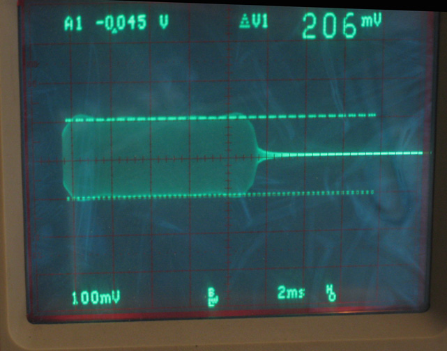
And here's the Exciter RF with its tank properly adjusted:
(Click on image to enlarge)

(Exciter RF waveform measured at the front-panel BNC, J6, using a Tektronix
TDS320 scope (100 MHz bandwidth).)
Schematics.
There are four pages. Here they are:
(Page 1. Click on image to enlarge)

Notes on page 1: This page is essentially the same as the original design, but
changes are:

- DC Voltage for IRF530s changed from 26 VDC to 12 VDC.
- 510 pf added to tank circuit (3570 pf total) so that the Tank circuit, when operating at 3.87 MHz, is properly tuned with Tuning Capacitor C11 at about half-mesh.
(Page 2. Click on image to enlarge)

Notes on page 2:
No change from the original circuit. But because the LM2576
switching-regulator now must deliver an additional 800 mA (or so, to power the
PA FETs), the inductor L3 really should be changed from 1000 uH to 470 uH or
330 uH. But it seems to run fine with the original value of 1000 uH, so I'll
leave modifying this for another day.
And, strictly speaking, I didn't need to incorporate a sequencer into the
Exciter's design -- I could have used the existing sequencer in the 813
transmitter to perform the same function. But incorporating this sequencer
allows me to easily test the Exciter as a stand-alone unit.
(Page 3. Click on image to enlarge)
 Notes on page 3:
This is the audio driver which drives the 813 Modulator Deck. Externally, and
prior to this stage, I use a
Behringer Xenyx 802 mixer/amplifier
to amplify and equalize my microphone.
For 100 percent modulation, the Modulator Deck requires an input level of
about 80 volts RMS (when driven with a sine-wave -- this is about 226 Volts
peak-to-peak). The simplest way to get this sort of amplitude is with a
transformer. On eBay I found an audio output transformer (designed to present
to a push-pull driving stage a load of 6.6K or 8K ohms when driving either a
4, 8, or 16 ohm load -- its Part Number is OT20PP), and I decided to connect
it in reverse to drive my Modulator Deck so that I could transform the
high-impedance of the Modulator Deck input to a low-impedance, and then drive
this low-impedance with a speaker amplifier designed to drive loads in the 4
to 16 ohm range.
To test which combination of input/output windings would work best in my
application, I connected the transformer to the Modulator Deck and drove it
with a stereo amplifier. With a 1 KHz sine-wave test signal, for full
modulation (corresponding to an audio drive of about 80 Vrms into the
Modulator deck), I needed about 12 Vpp of drive from the stereo amp.
For the actual transformer driver, I used an LM1875 speaker amplifier. Its
output is single-ended, so, to get 12 Vpp out with some headroom, I used the
26 VDC power supply to power it.
I also decided to use the 16 ohm tap as the primary (driven by the LM1875) and
the 6.6K ohm taps as the secondary (to drive the Modulator Deck). This is the
lowest step-up turns-ratio provided by the windings, and the Modulator Deck's
input impedance is transformed to be about 5.4 ohms, as measured at the output
of the LM1875, which conveniently lies between the LM1875's 4 ohm and 8 ohm
load specs. (Any other combination of windings would have resulted in a lower
load impedance for the LM1875).
When driving the Modulator Deck to full modulation, the LM1875 delivers about
3.6 watts into this 5.4 ohm load.
There is a potentiometer to allow some amount of gain adjustment, but the
primary gain is back at the Behringer mixer. And there's a mute circuit to
mute the audio drive to the Modulator Deck when the 813 Transmitter is
not transmitting. (The 813 transmitter does not like it when the modulator and
modulation transformer are driven when the PA deck is
not
generating RF).
The low-frequency -3 dB point is about 280 Hz (determined by R28 and C44),
which I purposefully added when I discovered that lowering this frequency
caused the AM signal to sound a bit fuzzy (due to IMD products related to the
voice frequencies below this point). The upper -3 dB point for the exciter/813
rig (combined) is around 4 KHz. These points were measured by driving the
modulator with sine-waves and measuring the peak-to-peak envelope of the
modulated RF.
As a precaution against EMI problems involving RF interacting with the audio
components, the audio components are all placed within a separate shielded
chamber (made using double-sided PCB stock) within the chassis. All signals
which transition into this chamber from the area containing the Exciter's RF
stages are first filtered using feed-thru caps and L/C (or R/C) low-pass
filters.
(Page 4. Click on image to enlarge)

Notes on page 4:
- The 26 VDC power supply is a Cosel 24V supply (adjustable +/- 10%), rated at 4.5 ADC that I picked up from eBay. Now that I've discovered that I don't need 40 watts of RF power, this supply could actually be rated at a much lower DC output current, but hey, hindsight is 20/20.
- The AC Connector and AC Line filter are actually an integrated modular unit.
- The VFO is an N3ZI DDS2 VFO. Its output is only about 380 mVpp, so I bump it up to about 2 Vpp (to drive the 'HC86 XOR gates) with an OPA690 op-amp. The 50 ohm resistor in series with the output was added to reduce some high-frequency ringing I had observed, but I'm not sure it's really needed -- I may have been mistaken in this measurement.
- The VFO Amp is only turned-on when transmitting. With the chassis buttoned-up, I've found that, even though the DDS VFO is always active (even during receive), I cannot hear it on my receiver.
- The Drain Current meter is 1.5 mA full-scale. The resistors (and sense-resistor) scale the current reading so that the meter represents actual current ÷ 2000.
- For adjusting the Tank's tuning capacitor, I added an RF tap (R32 and R33) which connects to a BNC on the front panel. The series-2K ohms represented by R32 and R33 help to isolate the tank circuit from the capacitance of coax-cables used to connect this BNC to a scope.
- And a diplexer is still used to help clean up the Exciter's RF output. The 50 ohm load for the Diplexer's parallel L-C circuit (i.e. the load for out-of-band frequencies) is actually seven 357 Ω, 1/4 watt resistors in parallel. And I placed the series L-C part of the diplexer in a Pomona box because I was concerned that, if not shielded, unwanted RF components would couple around it to the output.
(Click on image to enlarge)

And here are some photos!
The Audio stage. Note the shielded compartment. And the LM1875 amplifier
attached to the side of the chassis for heatsinking.
(Click on image to enlarge)

In the rack and on the air!
(Click on image to enlarge)

(Note: This shot was taken with the FETs powered with 26V, rather than 12V,
and a 6 dB attenuator between the Exciter and the PA Deck. With a 12V FET
power source, the meter needle is about 0.4 mA (out of 1.5 mA FS),
representing about 0.8 Amps of Drain current.
Additional Notes:
Because the tank transformer is 1:1, I wondered what the effect would be
if I moved the Tuning Capacitor (C11) from the primary side of the tank to the
secondary side. This would allow me to more easily mount the cap, because it
no longer would need to float. However, when I performed this experiment, I
discovered two issues:
- The tuning range narrowed.
- Output power varied slightly with frequency.
Resources:
Datasheets:
Caveats:
1. I could have easily have made a mistake, so please regard (and use) this
design accordingly.
2. High voltages can kill. Use caution.