I rely on Smith Charts to help understand how L-networks match an unknown impedance to our "target" impedance (i.e. Zo). If Smith Charts and Reflection Coefficients are unfamiliar or you are rusty with them, I would recommend taking a quick look at my post: A Brief Tutorial on Smith Charts. The important points mentioned in it are:
First, a load's Reflection Coefficient, Γ (Gamma) can be plotted on the complex-plane. This plotted point will have a magnitude (also known as ρ (rho)), when referenced to the center of the plane (0,0), that is between (and inclusive of) 0 and 1.
Second, the Smith Chart itself is simply an overlay over this plot of the Reflection Coefficient, and this overlay identifies the impedance (or admittance) of the load associated with Γ at any point.
Third, if we add capacitance or inductance in series with our load we can visualize this as moving Γ along the Smith-Chart's circles of constant-resistance (the direction will depend on the sign of the reactance: inductive or capacitive). And in an analogous fashion, if we add capacitance or inductance in parallel with our load, we will move Γ along circles of constant-conductance.
Fourth, when we add capacitance or inductance to our circuit, this movement of Γ (and thus the change in impedance or admittance) is only along these circles. It is not along the other lines representing constant-reactance or constant susceptance.
Fifth, circles of constant SWR can be plotted on the Smith Chart. These circles are centered at (0,0) -- the chart's Zo, and their radius is ρ, the magnitude of Γ.Finally, before we start, this is a lengthy post and it really consists of two main sections:
The first section describes the eight L-Match networks, how they work (Smith Charts), and how they can be used (and I explain a common misconception regarding when series-parallel networks should be used).
The second section deals with actual simulations of the four most commonly used L-networks. The simulations cover power loss, peak voltage across components, current through components, and component values.
Section 1: L-Network Impedance Matching
First, a definition:
Zload = Rload + jXload
And second: I will often refer to the "target" impedance that we want to match to as Zo. Assume, for this post, that Zo = 50 ohms.
I hope it's obvious from my Smith Chart discussion (A Brief Tutorial on Smith Charts ) that if our load has a reflection coefficient that lies on a Smith Chart's "circle of constant resistance" that intersects the point (0,0) in the complex plane (and only one constant-resistance circle will intersect this point -- it's the circle representing R = Zo), we can easily match the load to our target impedance by adding a single appropriately-valued capacitor or inductor in series with our load.
Similarly, if Zload's Γ lies on a "circle of constant conductance" that intersects the point (0,0) in the complex plane (and only one constant-conductance circle will intersect this point -- it's the circle representing G = 1/Zo), we can easily match the load to our target impedance by adding a single appropriately-valued capacitor or inductor in parallel with our load.
(click on image to enlarge)

And, of course, if the load's reflection coefficient is already at (0,0) on the complex plane, no additional matching is required.
But for all other possible reflection coefficients on the complex plane, we will need more than one reactive component to match our load to our target impedance.
Of course, we can use any number of components to create this match, but, it turns out, a minimum of two reactive components is sufficient to match a load to our target impedance (and for the purposes of this discussion I'm going to avoid components such as transformers and stick with just capacitors and inductors).
There are eight possible networks that use a total of two reactive components, and these configurations all have a circuit topology that looks like an "L" (if turned sideways and sometimes flipped). Thus, the name "L-network."
The eight networks are shown in the drawing below:
(click on image to enlarge)

In the drawing above I've paired these networks into "duos." For example, configurations 1 and 2 form a duo because each network consist of a series capacitance and a parallel inductor (i.e. CsLp or LpCs). Throughout this post I will refer to configurations that share the same type of component for their series element and the same type of component for their parallel element as duos. From the chart above, there are four "duo" pairings:
CsLp / LpCs
LsCp / CpLs
LsLp / LpLs
CsCp / CpCs
Continuing on...
Each of the eight L-network configurations can be used to transform an unmatched impedance to a matched impedance, and each do this either by first transforming Zload's impedance into an intermediary impedance whose Γ lies on the Smith Chart "circle of constant-resistance" representing R = Zo (e.g. 50 ohms), or by first transforming Zload's impedance into an intermediary impedance which lies on the Smith Chart "circle of constant-conductance" representing G = 1/Zo (e.g. 0.02 Siemens).
The L-network component nearest the load performs this transformation to an
impedance on either of these two circles. And, if we were to move from
the load towards these two "target" circles by incrementally changing this
component, we would find that the changing intermediary impedance moves along
paths consisting of other constant-resistance or constant-conductance
circles.
The next component (the one closest to the source), then transforms the intermediary impedance (or admittance -- you can think of it as either) to our destination Zo. This transformation essentially moves the impedance along either the R=Zo circle or along the G=1/Zo circle until it reaches the center of our Smith Chart (coordinate (0,0) on Γ's complex plane) -- our match point!
The diagram below shows how each of the eight L-network configurations can transform Zload first along a circle to one of two circles (constant-resistance or constant conductance) that intersects the center of the chart, and then finish the transformation by moving the impedance from that intermediary point, along this circle (either the R=Zo or G=1/Zo circle), to the center point (0,0) of the chart. The image below illustrates this:

Note that the impedance (and thus Γ) always moves along one circle or another (were we to incrementally change its reactance or susceptance). It does not move along the other (non-circle) lines that represent constant-reactance or constant-susceptance. (Although in real-life there might be some small amount of movement along these other lines, due to resistive loss in real-life inductors and capacitors).
Although the diagram above shows the Smith Chart divided into eight "regions" and a different L-Network in each, L-Networks can actually be used across multiple regions. But some are more useful than others, in that some can match impedances over a larger Smith Chart area than can others.
The dual-inductor and dual-capacitor networks are limited in the regions they cover. For example, let's look at the LsLp / LpLs duo. First, matching with LsLp:

And matching with LpLs:

These two configurations can only match impedances within the bottom area of the Smith Chart (shown in yellow, below) and no where else:

In an analogous fashion, dual-capacitor networks also have limited usefulness because they, too, cannot cover the entire Smith Chart. Here's the region spanned by the CsCp and CpCs duo:

On the other hand, the LsCp / CpLs duo of networks can cover impedances on the entire Smith Chart, as shown below, where one network covers the yellow region and the other network covers the unshaded region:

(Note that I call the LsCp / CpLs duo "Low-pass" L-networks because, ostensibly, they provide a low-pass function while also impedance matching, although the amount of filtering they actually provide depends upon Zload's impedance).
Similarly, the CsLp / LpCs duo of "High-pass" L-networks can also cover impedances on the entire Smith Chart:

Clearly, if we're going to design an antenna tuner based upon L-networks, then using either the LsCp / CpLs combination or the Cs/Lp / LpCs combo is the way to go -- we can cover the entire Smith Chart with an inductor and a capacitor and a switch (to flip the chosen configuration between series-parallel and parallel-series).

The next component (the one closest to the source), then transforms the intermediary impedance (or admittance -- you can think of it as either) to our destination Zo. This transformation essentially moves the impedance along either the R=Zo circle or along the G=1/Zo circle until it reaches the center of our Smith Chart (coordinate (0,0) on Γ's complex plane) -- our match point!
The diagram below shows how each of the eight L-network configurations can transform Zload first along a circle to one of two circles (constant-resistance or constant conductance) that intersects the center of the chart, and then finish the transformation by moving the impedance from that intermediary point, along this circle (either the R=Zo or G=1/Zo circle), to the center point (0,0) of the chart. The image below illustrates this:
(click on image to enlarge)
Note that the impedance (and thus Γ) always moves along one circle or another (were we to incrementally change its reactance or susceptance). It does not move along the other (non-circle) lines that represent constant-reactance or constant-susceptance. (Although in real-life there might be some small amount of movement along these other lines, due to resistive loss in real-life inductors and capacitors).
Although the diagram above shows the Smith Chart divided into eight "regions" and a different L-Network in each, L-Networks can actually be used across multiple regions. But some are more useful than others, in that some can match impedances over a larger Smith Chart area than can others.
The dual-inductor and dual-capacitor networks are limited in the regions they cover. For example, let's look at the LsLp / LpLs duo. First, matching with LsLp:
(click on image to enlarge)
And matching with LpLs:
(click on image to enlarge)
These two configurations can only match impedances within the bottom area of the Smith Chart (shown in yellow, below) and no where else:
(click on image to enlarge)
In an analogous fashion, dual-capacitor networks also have limited usefulness because they, too, cannot cover the entire Smith Chart. Here's the region spanned by the CsCp and CpCs duo:
(click on image to enlarge)
On the other hand, the LsCp / CpLs duo of networks can cover impedances on the entire Smith Chart, as shown below, where one network covers the yellow region and the other network covers the unshaded region:
(Click on image to enlarge)
(Note that I call the LsCp / CpLs duo "Low-pass" L-networks because, ostensibly, they provide a low-pass function while also impedance matching, although the amount of filtering they actually provide depends upon Zload's impedance).
Similarly, the CsLp / LpCs duo of "High-pass" L-networks can also cover impedances on the entire Smith Chart:
(click on image to enlarge)
Clearly, if we're going to design an antenna tuner based upon L-networks, then using either the LsCp / CpLs combination or the Cs/Lp / LpCs combo is the way to go -- we can cover the entire Smith Chart with an inductor and a capacitor and a switch (to flip the chosen configuration between series-parallel and parallel-series).
Calculating Actual Component Values
How can we calculate L-Network component values?
One way is to use a Smith Chart. If we know the load's complex impedance, we can quickly come up with an L-network to match it to our target impedance. Programs such as Smith V3.10 are a great tool for doing this and will give us actual component values.
But if we're trying to discover a range of values to match a corresponding range of load impedances and SWRs, determining component values via a Smith Chart quickly becomes tedious. Can we instead use a formula to calculate values?
If you take a look on the internet, you'll come across at least two different ways to calculate L-network component values:
The first method uses Q. Here's an example: http://www.ece.ucsb.edu/~long/ece145a/Notes5_Matching_networks.pdf
Personally, I don't use this method and I'm also not sure that it is an all-encompassing technique. Note that the load is assumed resistive. What happens if the load is complex, which it could easily be?
Also, this technique requires that the source resistance, Rs, be known (e.g. the 2011 edition of the ARRL Handbook states that "To design an L-Network, both source and load impedances must be known.")
Unfortunately, the source impedance is not always known.
For these reasons, I prefer the second technique for calculation L-network component values. It can be used with any complex load impedance, and it is independent of the source impedance.
This second technique uses two sets of equations. You can find the derivation of these equations here, for example: http://www.ece.msstate.edu/~donohoe/ece4333notes5.pdf.
I'll get to these equations in just a bit, but first...
A slight digression into a common misconception...
Practically every reference that I've come across states that one should select series-parallel versus parallel-series networks per the following conditions:
If Rload > Zo: Use series-parallel configurations such as LsCp or
CsLp.
If Rload < Zo: Use parallel-series configurations such as CpLs or
LpCs.
For example, here's an image from the ARRL Handbook for Radio Communications, 2011 (figure 20.9, page 20.10) showing just that (although they use Rs in lieu of Zo):
(click on image to enlarge)

But there's a problem...
The Rload > Zo constraint is incorrect. In fact, it is too constraining. Series-parallel networks (e.g. LsCp or CsLp) can be (and are) used in other regions in the Smith Chart and not just when Rload > Zo.
Let me repeat that:

(This misconception seems to be very common, and I'm just using the page from the ARRL Handbook (2011) as an example. One can easily find many other examples which repeat this same misconception).
The Correct Constraint:
The correct constraint can be expressed two ways:
Gload < 1/Zo
or
Rload + (Xload2
/ Rload ) > Zo
The two are equivalent:

Note: this corrected constraint only determines if a series-parallel network can transform a specific load impedance. This network could be low-pass or high-pass, given the load impedance (but it won't be both).
Similarly, the constraint for parallel-series networks, RL < RS, determines if a parallel-series network can transform a specific load impedance, but it does not specify if the matching network will be low-pass or high-pass. (It will be one or the other, but it won't be both.)
Update
7 April 15
I've given this topic its own blog post.
For a more detailed explanation, go here:
Okay, on to the simulations!
Section 2: L-Network Simulations
Simulation Methodology:
I've created an Excel spreadsheet to let me analyze and compare the various L-Network configurations. (Excel handles complex number calculations, but those of you who are more comfortable with, say, Matlab, could use it to do the same thing).
The Excel spreadsheet calculates the following:
- Component values of the L-network, based upon reactances calculated by the spreadsheet given Operating Frequency, SWR, and L-network configuration.
- Equivalent-Series-Resistance (ESR) in each matching-network inductor and capacitor, given pre-defined Q's and the spreadsheet's calculated component reactances.
- Reflection Coefficient, as seen by the source (and modified by component ESR).
- Power dissipated (as a percent of total power) by all ESRs and by the load.
- Peak-voltage-across and current-through each L-Network Component (ditto for the load).
Power Dissipation in LsCp / CpLs and CsLp / LpCs Matching Networks:
Let's calculate inductor power dissipation for the CsLp / LpCs duo and for the LsCp / CpLs duo. Is there any difference in power dissipation between the inductor being placed in series versus in parallel? (I'll use a high SWR to accentuate any differences).
The simulation conditions are:
- Frequency = 3.5 MHz
- Zo = 50 Ohms
- SWR = 32:1
- Capacitor Q (Qc) = 2000
- Inductor Q (Ql) = 100
- Power = 1000 watts
(click on image to enlarge)

First, some notes regarding the plot above:
The X-Axis corresponds to the angle of Zload's Γ (Reflection
Coefficient) when expressed in Polar Coordinates (ρ, theta).
To create these plots Excel increments this angle in 2 degree increments
around a Smith Chart's "circle of constant SWR" (thus keeping
ρ fixed,) starting on the Smith Chart's right-hand x-axis (i.e.
theta = 0 degrees) and rotating through a full 360 degrees.
And as we go around the circle, Excel's equations will be switching from one configuration of a duo to the duo's other configuration as we pass into the Smith Chart area for that configuration (e.g. LsCp will flip to its corresponding CpLs configuration and then back again later).
And now, a couple of observations on the plot above:
Here's the same plot, but at an SWR of 4:1. Note the interesting symmetry of the power-dissipation curves around 90 degrees and 270 degrees.

Now let's now take a look at capacitor power dissipation:
Again, the simulation conditions are:

Observations:

If Qc equals Ql, capacitor power loss and inductor power loss have the same peak value:

...and here's total L-network power loss, for the same Qc = Ql condition:

Conclusion 1:
So power-dissipation is not a differentiating factor when designing a general-purpose tuner.
Let's now look at...
Component Current and Peak-Voltage in LsCp / CpLs and CsLp / LpCs L-Networks:
Using the same Excel spreadsheet I've calculated the peak-voltage across each component as well as the current through them. Again, the simulation conditions are:
(click on image to enlarge)

(click on image to enlarge)

And as we go around the circle, Excel's equations will be switching from one configuration of a duo to the duo's other configuration as we pass into the Smith Chart area for that configuration (e.g. LsCp will flip to its corresponding CpLs configuration and then back again later).
And now, a couple of observations on the plot above:
- Maximum inductor power dissipation (as a percentage of total power) is the same irrespective of configuration. That is, matching networks with their inductor-in-series and matching networks with their inductor-in-parallel both have the same max dissipation when measured around the entire constant-SWR circle!
- Maximum inductor power dissipation peaks at roughly 270 degrees (i.e. -90 degrees) and is high from (very roughly) 180 degrees to 360 degrees.This is the lower region of the Smith Chart: Rload < Zo and Xload has capacitive reactance.
- If designing to match a known load impedance in a particular "Γ angle" pie-slice region of the Smith Chart, note that one configuration might have lower power dissipation than the other.
Here's the same plot, but at an SWR of 4:1. Note the interesting symmetry of the power-dissipation curves around 90 degrees and 270 degrees.
(click on image to enlarge)
Now let's now take a look at capacitor power dissipation:
Again, the simulation conditions are:
- Frequency = 3.5 MHz
- Zo = 50 Ohms
- SWR = 32:1
- Capacitor Q (Qc) = 2000
- Inductor Q (Ql) = 100
- Power = 1000 watts
(click on image to enlarge)
Observations:
- Peak power dissipation is the same regardless of the capacitor being a shunt element or a series element.
- Again, note the symmetries around 90 and 270 degrees.
- And note how the capacitor power dissipation has the same shape as the inductor power dissipation for the same SWR (32:1). It's just that the peak power is scaled down and the maximum is around 90 degrees, rather than around 270 degrees.
- If designing to match a known load impedance in a particular "Γ angle" pie-slice region of the Smith Chart, note that one configuration might have lower power dissipation than the other.
(click on image to enlarge)
If Qc equals Ql, capacitor power loss and inductor power loss have the same peak value:
(click on image to enlarge)

...and here's total L-network power loss, for the same Qc = Ql condition:

Conclusion 1:
When considering all loads possible for a particular SWR, there is no difference in inductor maximum power dissipation between the CsLp / LpCs configuration duo and the LsCp / CpLs configuration duo, nor in capacitor power dissipation between these two duos, given equivalent component Q's. Both result in the same component power dissipation, but at different Reflection Coefficient angles (relative to the positive x-axis) when comparing one duo to the other.
So power-dissipation is not a differentiating factor when designing a general-purpose tuner.
Let's now look at...
Component Current and Peak-Voltage in LsCp / CpLs and CsLp / LpCs L-Networks:
Using the same Excel spreadsheet I've calculated the peak-voltage across each component as well as the current through them. Again, the simulation conditions are:
- Frequency = 3.5 MHz
- Zo = 50 Ohms
- SWR = 32:1
- Capacitor Q (Qc) = 2000
- Inductor Q (Ql) = 100
- Power = 1000 watts
First, a plot of Peak-Voltage:
And here, Current:
They might be a bit difficult to figure out. So here's a table listing the maximum values for each:

The plots above were for an SWR of 32:1. What happens to them if the SWR is lower, say, 4:1? Let's take a look
First, a plot of Peak-Voltage:

And here, Current:

And again, the maximums in tabular form:

Comments on the Voltage and Current Simulations:
- The plots are frequency-independent. This is because component Q, as defined for the simulations, is also frequency independent. In actual life, Q would probably vary with frequency (e.g. coil Q degrading at higher frequencies).
- If inductor-Q and capacitor-Q are identical, the peak power dissipated in each will be identical.
- If designing to match a known load impedance in a particular "Γ angle" pie-slice region of the Smith Chart, note that one configuration might have lower peak voltage or current than another.
When considering all loads for a particular SWR, there is little difference in Peak-Voltages or in Current between the CsLp / LpCs configuration duo (i.e. High-Pass network) and the LsCp / CpLs configuration duo (i.e. Low-Pass network). (What differences there are become more noticeable at high SWRs.)
So, component peak-voltage or current is not a deciding factor in choosing between the CsLp / LpCs and the LsCp / CpLs configurations for a general-purpose tuner.
So far the performance of the two configuration-duos is essentially equivalent. So let's look now at component values...
Component Values in LsCp/CpLs and CsLp/LpCs L-Network Tuners:
Again, using the EXCEL spreadsheet to calculate L-Network component values.
And again, the simulation conditions are:
- Frequency = 3.5 MHz
- Zo = 50 Ohms
- SWR = 32:1
- Capacitor Q (Qc) = 2000
- Inductor Q (Ql) = 100
- Power = 1000 watts
(click on image to enlarge)

That's interesting, there's an outlier!
Let's look at Inductor values:
(click on image to enlarge)

Another outlier!
If I calculate the maximum and minimum inductance and capacitance for these two networks, they are:

Note the huge maximum values required for the CsLp / LpCs High-Pass networks!
(Also note: Excel runs its calculations in discrete steps 2 degree increments, so the actual maxima and minima are probably a bit different from those listed in the table above, unless they happen to lie exactly on a 2-degree increment).
Let's lower the SWR to 4:1 and look at these component values again:
Inductance:
(click on image to enlarge)

Capacitance:
(click on image to enlarge)

At a 4:1 SWR, inductance for the High-Pass networks peaks at a Γ angle of about 52 degrees. And capacitance peaks at an angle of about 232 degrees. Let's take a look at what's going on...
First, let's look at what's happening at 52 degrees. Given the SWR of 4:1, let's plot this point on a Smith Chart:
(click on image to enlarge)

And now, plotting the path to a match:
(click on image to enlarge)

So what's going on?
Because this is the CsLp (High-Pass) network, we only need to move a small distance along a "circle of constant conductance" (conductance circle because we are adding a shunt component across the load -- in this case, inductance) to reach the R=50 "circle of constant resistance" (from which it will be a straight shot down to our match point).
A very small movement along a "circle of constant conductance" is equivalent to adding a very large reactance in parallel with the load. In the limit, if we added a parallel element of infinite ohms of reactance (i.e. an open-circuit) across Zload, there would be no movement along the constant-conductance circle. So, if we require only a very small movement along the constant-conductance circle, we need to add a relatively large reactance in parallel with Zload. For the CsLp network, this means a large inductor.
Let's do the same thing at the 232 degree Γ angle:
(click on image to enlarge)

Now we're looking at an LpCs (again, High-Pass) network. Given the position of the load on the Smith Chart, we only need to move a small distance along a "circle of constant resistance" (because we are adding a component in series with the load -- in this case, a capacitor) to reach the G=0.02 "circle of constant conductance" (from which it will be a straight shot up to our match point).
A very small movement along a constant-resistance circle is equivalent to adding a very small reactance in series. In the case of the LpCs network, the series element is a capacitor (and the movement is counter-clockwise), and for there to be a low reactance the capacitance needs to be relatively large.
(One way to look at this: in the limit, if our series element were a short circuit (zero ohms reactance), Γ would not move at all. That is, if we were already on the G=0.02 "circle of constant conductance" (so that no movement was first required along a "circle of constant resistance", there would be no series-capacitor at all -- it would be replaced with a short.)
This implies: if using the LpCs - CsLp High-Pass L-Network networks in an antenna tuner, one might want to add a switch to short out the capacitor (i.e. minimize series reactance) and change the inductor switch from single-pole double-throw to single-pole triple-throw (with the middle position disconnecting the inductor from the matching network -- maximizing parallel reactance).
Something like this:

(Note that vacuum-variable caps will often short at the "maximum capacitance" end of their travel, so no parallel-switch would be needed in that case).
So, we've determined that the LpCs / CsLp High-Pass networks can sometimes require very larger inductors and capacitors compared to the LsCp / CpLs Low-Pass networks, depending upon Zload.
What component-value drawbacks do the LsCp / CpLs Low-Pass networks have?
The spreadsheet calculations show that no large capacitor is required -- in fact, we have the opposite problem -- the closer Zload is to the R=Zo "circle of constant resistance", the smaller the capacitor must be to move the impedance along a "circle of constant conductance" to the R=Zo "circle of constant resistance (recall that for the CsLp High-Pass network the inductor had to be larger the closer Zload was to the circle).
Again, this is because we want the shunt element to have a very small effect on Zload; therefore, we don't want to change it much. And so the shunt element has to be a large impedance. If the shunt element is a capacitor, its value must be small for it to have a large impedance.
Similarly, the CpLs Low-Pass network has the opposite problem of the LpCs High-Pass network -- the closer Zload is to the G=1/Zo "circle of constant conductance", the smaller the inductor must be to move Zload onto that circle.
This is because we want the series element to have a very small effect on Zload -- we don't need to change it much. So the series element must have a very small impedance. In this case, the series element is an inductor, so it must have a very small inductance if the series-element's impedance is to be small.
So, whereas LpCs / CsLp High-Pass networks can sometimes require very large inductors and capacitors compared to the LsCp / CpLs Low-Pass networks (depending upon Zload), LsCp / CpLs networks can have very small inductors and capacitors compared to the LpCs / CsLp networks.
Here's a table of the maximum and minimum component values required to match an SWR of 4:1. Notice how the low-pass networks (LsCp/CpLs) have smaller minimum values than the high-pass networks.

At minimum inductance Γ's angle is around 128 degrees.
And at mimimum capacitance Γ's angle is around 308 degrees.
Below are the Smith Chart locations for Low-pass network minimum component values and High-pass network maximum component values (for SWR = 4:1):
(click on image to enlarge)

Let's continue the analogy with the High-Pass networks to its logical conclusion...
If the value of Ls and/or Cp of our components cannot be made small enough, we could add switches to 1) short out the inductor (i.e. replacing it with a short circuit which has minimal inductance), and 2) open the connection to the capacitor, making the resulting Cp capacitance very small, too.
Just like this:

Looks like the same switch configuration that I drew for the High-Pass duo, doesn't it?
Summarizing: overall, the High-Pass networks can have the largest value components if used as a general-purpose tuner. But -- when matching a specific impedance, sometimes a High-Pass network will have smaller component values than the Low-Pass network. As an example, consider the following Zload:
Zload = 5 - j400 @ 3.75 MHz
Either of these two networks can match this load to 50 ohms:
CpLs (Low-pass): C = 2550 pf, L = 17.6 uH
CsLp (High-pass): C = 33.4 pf, L = 12.9 uH
Note that the High-Pass network uses smaller components. So, although High-Pass networks can result in much larger component values at certain load impedances than Low-Pass networks, at other times their component values will be smaller than the equivalent Low-Pass network.
Jack Belrose, in his article "On the Quest for an Ideal Antenna Tuner," QST, Oct. 2004, describes a matching network that let's the user select any of the four networks (CsLp, LpCs, LsCp, CpLs) to get around this problem of network-specific "out-of-range" component values that can occur in different areas of the Smith Chart.
With that thought in mind, I created the following plot showing "allowed" networks if we limit their values to lie between maximum and minimum values.
(click on image to enlarge)
If we create the same plot at an SWR of 32:1 (in lieu of 4:1) to accentuate the differences between networks, we see something interesting:
(click on image to enlarge)

The component values of the High-Pass network are almost always lower than those of the Low-Pass network, except in those regions where the High-Pass network's capacitance or inductance values skyrocket.
On the other hand, for low SWR loads, the Low-Pass network uses smaller component values than do High-Pass networks. Here's how they compare at an SWR of 2:1
(click on image to enlarge)

So what does all of this mean?
To me it means that, if working with loads that have a high SWR, you're probably better off going with High-Pass network to keep component values down (except in the regions of skyrocketing values).
BUT: if you need to match Zloads where High-Pass network component values blow up, you will still need to use relatively large values of capacitance and inductance if implementing a Low-Pass network, but at least the component values are now realizable (to some extent). So, is there any advantage to a High-Pass L given that the Low-Pass network covers all the bases and doesn't blow up?
I don't know.
But this makes me wonder...can a High-Pass T-Network (which is essentially a High-Pass L-Network with an additional series-element) cover the full 360 degrees of an SWR circle with lower component values (in the range of the Low-Pass network or lower) and (roughly) the same amount of loss? In other words, can the High-Pass T-network cover the cases where the High-Pass L-network blows up?
Hmmm...something to explore!
Power Loss versus Inductance Value
In Conclusion:
If designing a general-purpose antenna tuner, I see little difference in power dissipation and component current and peak-voltages between the CsLp/LpCs High-Pass networks and the LsCp/CpLs Low-Pass networks. Instead, the main difference I see is with component values.
Note though, that at certain load impedances CsLp/LpCs High-Pass networks require much higher "maximum" values of inductance and capacitance compared to the LsCp/CpLs Low-Pass networks. But outside of the "blow up" impedances, the High-Pass network will often have lower component values than the Low-Pass networks for loads with high SWRs.
L-Network Extras...
1. I was wondering what the maximum component values would need to be for Low-Pass L-Networks if they were to be guaranteed to convert certain SWRs down to a 1:1 SWR match. Here's a table:

2. [Added 13 June 2015] I was recently wondering if there was a correlation between inductance value and power loss when using a Lowpass L-Network. That is, did power-loss increase as inductance increased (as we move around a Smith Chart's "Circle of Constant SWR" (and assuming inductance Q was far worse than capacitance Q)?
Well, not really, as you can see from the plot below:
(click on image to enlarge)

Max power loss occurs while inductance is increasing, rather than aligning with the inductance curves. So power loss does not correlate well with inductance.
BUT, there is useful information here, never the less...
Given a Lowpass L-network, maximum power loss occurs in the CpLs configuration (inductance in series with load).
And if in the LsCp configuration (which usually has lower power loss than the CpLs configuration), power loss does correlate with inductance value.
So, if you can adjust the length of your feedline, my opinion is: try to adjust it so that...
- The L-Network is in its LsCp configuration for as broad a frequency swath as possible (rather than the CpLs configuration), and
- The value of L is minimized.
(If you cannot do both of these, then I would shoot for one or the other. But it's difficult to say if you should minimize L in the CpLs configuration over choosing the LsCp configuration with a higher value of L. This decision really depends upon the Q (parasitic resistance) of the components being used)
3. More on LsCp/CpLs Power Dissipation [added 9/9/18]
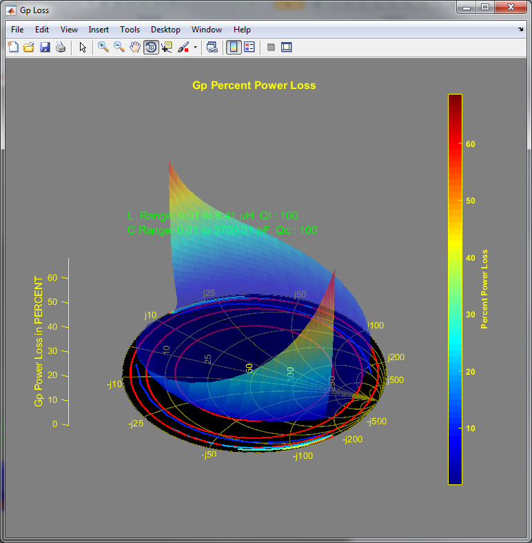
Dick Benson, W1QG, used his MATLAB programming skills to come up with a novel way to present L-Network loss -- in 3D!
A note regarding these plots: In addition to being 3D, contour lines are also plotted on the Smith Chart. These contours correspond to the 'ticks' on the vertical color bar to the right of the Smith Chart.
For example, in the first plot shown below, the contours represent 2, 4, 6, 8, 10, 12, 14, and 16 Percent Power Loss, which correspond to the tick-marks of the color bar at the right of the Smith Chart.I utilized Dick's work to plot loss along lines of constant-SWR, and the first group of plots below use this technique. Note that the largest SWR I plotted is 32:1 (which thus defines the outer circumference of the circle).
The first LsCp/CpLs plot shows total network loss assuming an inductor Q of 100 and capacitor Q of 2000:

Note that this dissipation is independent of frequency! It only depends upon the loss within the series inductor and the shunt capacitor.
In 3D, the power dissipation looks like:

Decreasing the capacitor Q from 2000 to 500:


And finally with both capacitor Q and inductor Q set to 100:


The following plots uses a MATLAB script Dick (W1QG) wrote to analyze L-networks. The first plot, below, shows the entire match-space given the following conditions:
- F = 3.5 MHz
- Inductor Range: 0.01 to 5.4 uH (21 steps)
- Capacitor Range: 0.01 to 3700 pF (37 steps)
- Qinductor = 100
- Qcapacitor = 1000
Match-space is found by calculating the exact load impedance that
a selected L and C (with their own internal losses -- i.e. Q) will tune
to a 1:1 SWR.
Note that this is not a trivial calculation. Many (if not
all) on-line Impedance Matching Network Design" sites assume that the
matching components are lossless (e.g.
here). As you will see in the plots, below, the worse the loss
of the L and C matching components, the greater will be the divergence
between the load values for a given pair of L and C values.

(Note that the component value ranges I've chosen are those I used for my Autotuner).
There are four separate match-space plots shown on the Smith Chart, above. Two of these compare the LsCp network against a lossless (Q = infinite) LsCp network. The other two compare the CpLs network against a lossless CpLs network.
Note how close lossy and lossless meshes are.
And the plots below show network power loss over the same match-space.


(Information on plotting Smith Chart data in 3-D can be found here: https://k6jca.blogspot.com/2018/09/plotting-3-d-smith-charts-with-matlab.html)
Changing the Q of the capacitor from 1000 to 100, I will repeat the same plotting process:

Note that the lossless and lossy meshes have diverged more (but they are still fairly close).
And here are the network power dissipation plots. Note the symmetry now that Qinductor equals Qcapacitor.

What do these plots tell us about actual measurements of network power loss?
It is always worthwhile comparing simulated results to actual real-world measurements. Simulated results will give you an idea of how a network (as modeled) should behave, but the actual measurements will take into account losses and parasitic elements that likely were not included in the simulation model.
To make real-world loss measurements, I have a collection of resistive loads (5, 10, 16.7, 50, 150, 250, and 500 ohms). These values correspond to SWRs of 10:1, 5:1, 3:1, and 1:1. And, being resistive only loads (with minimal reactance), I can use them for loss measurements on all the HF ham bands.
When I designed my L-Network Autotuner, I measured its loss for Zloads of 5+j0 and 500+j0 ohms, which represent its worst-case spec'd SWR (10:1). Did my measurements accurately reflect worst-case power loss for any load with a 10:1 SWR?
Let's try to answer this question with a MATLAB simulation. Note that I've made Qc equal to Ql, and both are 100, for illustration purposes.


As you can see in the plots, measuring loss with loads of 5 and 500 ohms does not represent worst-case loss! Worst case loss is not when rho has an angle of 0 or 180 degrees (i.e. loads are resistive with no reactance), but instead, for the example above, maximum loss occurs for rho angles of 66 and 246 degrees where the load impedance is complex.
So -- should I create loads for these "worst-case" complex impedances?
Well...I suppose I could, but because these impedances are complex, although the reactance would not change on a band-by-band basis, the actual inductance or capacitance values representing this reactance would be different for each band -- indeed for each frequency.
That would be a lot of loads to fabricate! Until I find a better method, I think I will stick with the handful of resistive loads that I already have.
Other Stuff...
1. A Note on my EXCEL Simulations:
It's quite possible that there are errors in my spreadsheet. However, I've compared my results to the L-Network simulations displayed by W8JI on his Antenna Tuners webpage, and they concur. (Although, please note: there is a mistake in W8JI's first L-network simulation (1.8MHz, load = 15+j0) -- it states that the coil Q is 200. However, the results are actually for a coil Q of 250).
So I feel fairly confident in my simulations, but there could always be a mistake -- it is a very large spreadsheet, after all, so the possibility for error is there. Please let me know if you come across one!
2. Resources:1. A Note on my EXCEL Simulations:
It's quite possible that there are errors in my spreadsheet. However, I've compared my results to the L-Network simulations displayed by W8JI on his Antenna Tuners webpage, and they concur. (Although, please note: there is a mistake in W8JI's first L-network simulation (1.8MHz, load = 15+j0) -- it states that the coil Q is 200. However, the results are actually for a coil Q of 250).
So I feel fairly confident in my simulations, but there could always be a mistake -- it is a very large spreadsheet, after all, so the possibility for error is there. Please let me know if you come across one!
You can download the Smith-chart software that I've used to make the Smith-Chart plots in this blog post from this site: Smith V3.10
W9CF T-Network Tuner Simulation. This simulator can also be used to calculate power-loss in High-Pass L-Networks. To do this, you can manually force the high-pass T-Network into a high-pass L-Network by setting one of the capacitors to a very large capacitance (i.e. low-reactance) value. Find the component values with, say, a Smith Chart. Then you can enter these values into the simulator by turning the simulator's knobs. Time consuming if you want to test a lot of values, but a good check if, say, you want to verify that your simulations are in the ballpark.
Impedance Matching Network Designer This is a useful tool for calculating L-network impedances. Let Rs = Zo and then enter in your load impedance. Interestingly, it correctly applies series-parallel configurations even when Rload is less than Zo (e.g. a load of 25+j50 at 3.5 MHz returns an LsCp network of 2.8uH and 1.2nF) in addition, of course, to applying a parallel-series LpCs network.
3. My Related Posts:
A quick tutorial on Smith Chart basics:
http://k6jca.blogspot.com/2015/03/a-brief-tutorial-on-smith-charts.html
Plotting Smith Chart Data in 3-D:
http://k6jca.blogspot.com/2018/09/plotting-3-d-smith-charts-with-matlab.html
The L-network:
http://k6jca.blogspot.com/2015/03/notes-on-antenna-tuners-l-network-and.html
A correction to the usual L-network design constraints:
http://k6jca.blogspot.com/2015/04/revisiting-l-network-equations-and.html
Calculating L-Network values when the components are lossy:
http://k6jca.blogspot.com/2018/09/l-networks-new-equations-for-better.html
A look at highpass T-Networks:
http://k6jca.blogspot.com/2015/04/notes-on-antenna-tuners-t-network-part-1.html
More on the W8ZR EZ-Tuner:
http://k6jca.blogspot.com/2015/05/notes-on-antenna-tuners-more-on-w8zr-ez.html (Note that this tuner is also discussed in the highpass T-Network post).
The Elecraft KAT-500:
http://k6jca.blogspot.com/2015/05/notes-on-antenna-tuners-elecraft-kat500.html
The Nye Viking MB-V-A tuner and the Rohde Coupler:
http://k6jca.blogspot.com/2015/05/notes-on-antenna-tuners-nye-viking-mb-v.html
http://k6jca.blogspot.com/2018/08/notes-on-antenna-tuners-drake-mn-4.html
Measuring a Tuner's "Match-Space":
Measuring Tuner Power Loss:
http://www.w8ji.com/antenna_tuners.htm (Good information on tuners. Check out the Q info for roller inductors)
http://www.ece.msstate.edu/~donohoe/ece4333notes5.pdf (Excellent derivation of equations for synthesizing L networks. But note the repetition of the error of when to use series-parallel networks. It's not just when Rload > Zo).
http://www.g3ynh.info/zdocs/z_matcing/part_1.html (Lots of interesting stuff on this site. Well worth the read. And it was this series of posts that got me thinking of impedance matching in terms of conductance, G.).
http://www.nonstopsystems.com/radio/pdf-ant/article-antenna-ideal-ATU.pdf (Belrose article from October, 2004 QST)
W0QE: Antenna Tuner Paper: http://www.w0qe.com/Papers/Antenna_Tuners.pdf
Standard Caveat:
I could have easily made a mistake anywhere in this blog post. If something looks wrong, is unclear, or doesn't make sense, please feel free to contact me!