
Summary: This post presents a new method for measuring impedances (e.g. impedances of Common-Mode Chokes) using a 2-port VNA and its S11, S21, S12, and S22 measurements. This method is an improvement over the G3TXQ method (described below), in that it is not susceptible to parasitic shunt impedances (and in addition, it will give values for those shunt impedances). I would like to thank Dick Benson, W1QG, who introduced me to this method and whom I consider to be its "father".
But before I describe this new method of measuring impedance with a VNA, let me backtrack and first discuss how Common-Mode impedance had been measured previously...
In a previous blog post I discussed two different ways to measure a Common-Mode Choke's impedance using a VNA: either (1) as a one-port measurement (using S11), or (2) as a two-port measurement, using S21, as described here by G3TXQ. I'll refer to this latter technique as the "S21 method".
For Common-Mode chokes used in RF applications, stray test-fixture capacitance (which might be only a few pF) can resonate with the choke's inductance and greatly change impedance measured via S11 (see my earlier blog post, here).
The plots below demonstrate this effect:

You can see that there is a large difference between a CM Choke impedance measured via S11 versus the same choke's impedance measured using the S21 method.
But how accurate is the S21 method? How do we know that its results aren't skewed, too?
Let's examine more closely the cause of this difference, because it will lead us to a third way of measuring a choke's impedance, Dick Benson, W1QG's, "Y21 Method."
Dick's method will show that the G3TXQ S21 method is actually pretty good (although its results can be influenced by parasitic shunt capacitances). And Dick's Y21 method, in addition to calculating a choke's impedance, will also give us the values of parasitic shunt capacitances that explain the resonate frequency shift when measuring impedance with S11.
Parasitic Impedances and the S21 Measurement Method:
The formula derived for G3TXQ's S21 measurement method is based upon the following schematic diagram (from G3TXQ's website) representing a VNA's two ports and the "Device-Under-Test" (i.e. DUT) connected between the two ports:

From this schematic representation (and using the definition of S21), we can derive the following equation expressing the DUT's impedance (Zdut) as a function of S21:
Zdut = Zo*((2/S21) - 2)
where Zo is typically 50 ohms (the VNA's designed-for impedance).
(For equation derivation, refer to this blog post: http://k6jca.blogspot.com/2018/06/transmit-common-mode-chokes-11-current.html )
From the schematic representation, above, how different would we expect an impedance derived from an S11 measurement to be from the impedance derived from S21?
From inspection of the schematic, Zin of the network (as seen from the perspective of the output of VNA Port A) should simply be the series connections of Zdut and the 50 ohm termination at VNA Port B. In other words: Zin = Zdut + 50.
I've modeled this with the dashed Yellow line, below:

But the actual Zin, as calculated from the measured S11, is the orange line. There is a huge difference between the two!
How to explain this difference? A reasonable explanation would be that the schematic representing the G3TXQ test fixture does not represent reality -- it isn't taking into account parasitic shunt capacitance at either of the test fixture.
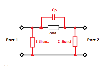
Let's assume that there are parasitic shunt impedances at each port, as shown, below:

(The shunt impedances are actually distributed capacitances, rather than lumped elements shown in the schematic. But lumped-element modeling provides a good first-order approximation of the effect of distributed capacitance).
Assuming this new model is correct, is there a way to determine the values of these shunt impedances? And how do they effect the impedance measurements made with the G3TXQ S21 method or via S11?
Yes, there is a way to determine the values of the shunt impedances while simultaneously determining the impedance of the DUT, and it is via Dick's Y21 Method.
And when we have determined these impedances values, we can examine their effect on the S21 and S11 methods of measuring impedance.
Let's look at the foundation of the Y21 method...
The Two-port PI network:
When I initially discussed my measurement discrepancies with Dick Benson, he brought up the issue of shunt impedances and mentioned that there was actually a straightforward way to calculate the values of all three elements of a Pi Network from a VNA's four S-parameter measurements (i.e. from S11, S21, S12, S22).
First, let's represent the G3TXQ S21 Impedance Measuring Method as a two-port Pi network with two unknown shunt impedances and an unknown series impedance (the latter representing the device-under-test whose impedance we are trying to determine), as shown, below:

The three impedances of this two-port PI network can be represented as three admittances in a two-port PI Admittance Network:

Note that these three admittances are simply the inverse of the three impedances:
Dick pointed out that, mathematically, a 2-port PI Admittance network can be
represented by a 2x2 Admittance Matrix:

The elements of this matrix are mathematical expressions of Y1, Y2, and Y3:

So, if we can determine the values of the four elements of the Admittance Matrix (i.e. Y11, Y21, Y12, and Y22), then we can easily calculate the three unknown impedances of the Pi Network:
But how do we determine Y11, Y21, Y12, and Y22 from our VNA measurements?
MATLAB's RF Toolbox has the perfect function for converting an S-parameter matrix to a Y matrix: s2y(s_params,Zo)
where s_params is (in our case) the 2x2 S-parameter matrix from the VNA, and Zo is the characteristic impedance (e.g. 50 ohms).
And once this conversion is made, it is then straightforward to use the equations, above, to calculate the impedances of the DUT and the two shunt elements.
In other words, Dick's "Y21 Method" of impedance measurement relies upon the creation of an Admittance Matrix for the PI network, and the elements of this Admittance Matrix (derived from the PI network's measured S-parameters) can be used to calculate all three unknown impedances of the PI network.
The implementation of this technique is straightforward with MATLAB, as the following code illustrates:
That is all there is to it!
If you don't have MATLAB, you can still calculate the elements of the Admittance Matrix from measured S-parameter data, using the equations, below:
Y11 = (S22 - S11 - S11*S22 + S12*S21 + 1)/(Zo*(S11 + S22 + S11*S22 - S12*S21 + 1))
Y12 = -(2*S12)/(Zo*(S11 + S22 + S11*S22 - S12*S21 + 1))
Y21 = -(2*S21)/(Zo*(S11 + S22 + S11*S22 - S12*S21 + 1))
Y22 = (S11 - S22 - S11*S22 + S12*S21 + 1)/(Zo*(S11 + S22 + S11*S22 - S12*S21 + 1))
And with these four values, the step to calculating the three impedances is straightforward using the Admittance Matrix equations:
Or, we could just combine the above seven equations to give us equations for our
three unknown impedances in terms of S-parameters:
Note that the equations, above, for Y11, Y12, Y21, and Y22, and for Zdut, Z_Shunt1, and Z_Shunt2, (all expressed in terms
of S-parameters) were generated using MATLAB's Symbolic Math and the following MATLAB
Code:


You can see that the Y21 and G3TXQ methods give very similar results, with some divergence that increases at higher frequencies. Not surprisingly, the impedance measurement calculated from S11 is very different.
Determining the Values of the Shunt Impedances:
As I've noted, Dick Benson's Y21 method has an advantage over the G3TXQ S21 method in that it allows us to easily compute the values of the unknown shunt parasitic impedances from the values in the 2x2 Admittance Matrix.
Note that the shunt impedances are always in the form R + jX. In the examples I've measured, the reactive "X" components of the shunt impedances are capacitive (i.e. X is negative), as you can see in the plot, below.

Even at 30 MHz, the reactive component is significantly greater than the resistive component (by a factor of 50). (Note, too, that the resistive component is slightly negative. Don't know why, but I suspect it could be due to something like measurement tolerances, etc.)
Below are plots of the equivalent shunt capacitances for this Common-mode choke. I also show their averaged values, too:

Do the Measured Shunt Capacitance Values Explain the S11 Impedance Measurement Difference?
Let's verify that the shunt capacitance values found via the Y21 method explain the Zin curve derived from the network's S11 measurement.
There are two ways to do this, and I'll show both methods.
Method 1:
The first method uses Zdut found from Y21 and user-defined (i.e. defined by me) shunt capacitance values. With these values I will create the S-parameters for this new "simulated" Admittance Matrix, and then calculate Zin from S11. This "simulated" Zin should be close to the measured Zin that was calculated from the network's measured S11.
I'll start with a PI network model consisting of the series DUT (whose impedance has been found via the Y21 method) and two user-defined shunt capacitors. I'll set the value of the "input" shunt capacitor to be the average of the measured shunt capacitance (i.e. 2.35 pF).
And, to demonstrate that the output shunt capacitor has little effect on S11 (because it is a large reactance shunted by a comparatively very small resistance -- the 50 ohm termination at the VNA's Port -- the 50 ohm termination swamps the capacitive reactance and thus dominates), I'll set this second shunt capacitance to be 0 pF.
In other words, the two-port network model looks like this:

Note that in the simulation Port 2 of the above network will be terminated in 50 ohms (using MATLAB's gammain() function). This 50 ohms represents the 50 ohm termination of the VNA's Port 2.
So Zin is being calculated for this network:

Below are the plots of the actual measured S11 versus the simulated S11 (the simulation using the network, above). As you can see, the two S11 plots are essentially identical, thus demonstrating that the measured input shunt capacitance is the cause of the Zin (from S11) curve.

To demonstrate the insensitivity to C2 (the network's output shunt capacitor), I'll set it to 100 pF. You can see that the simulated curve remains essentially unchanged:

(Note -- the MATLAB code that calculates the Zin of the simulated network is listed in the block of code at the end of the next section, below).
Method 2:
The second method is essentially just the reverse of the first method.
I'll take the measured Zin (calculated from the measured S11), and from these Zin values, plus my user-defined capacitance values, I will derive Zdut. This Zdut should be close to the Zdut found via the Y21 method.
Again, I will assume that the network's output shunt capacitor has an insignificant effect (because it is a high impedance in parallel with 50 ohms -- the 50 ohms being the termination at the VNA's port 2).
And again, for simplicity, I will assume that the input shunt capacitor's value 2.35 pF -- the average of the values I measured from 1 to 30 MHz.
So the PI network becomes:

The equation for Zdut in terms of Zin is:
where Yshunt1 is the admittance of the 2.35 pF cap, i.e. 1/Zshunt1.
Here is the result:

The dashed green line is our derived-from-S11 Zdut value. It's close to the measured value, but not exact. What might be going on?
If I change the input shunt capacitor from 2.35 pf to 2.30 pf, the plots become:

There is a noticeable difference with only a 50 femtoFarad change in shunt capacitance. Interesting!
Recall from earlier in this post the plots of the measured shunt capacitances. The input shunt capacitance is the blue line:

Let's use these values to find Zdut instead of the fixed-value of 2.35 pF. Here's the result:

Looks very good! But how good? Let's zoom in on a section:

The derived-Zdut is essentially identical to the measured Zdut (showing two things: (1) the equation to calculate Zdut from Zin is correct, and (2) the output shunt capacitor has little effect).
But before I end this discussion, I'd like to make a quick note regarding this second method:
Note regarding Method 2:
When I first attempted to calculate Zdut from measured Zin values, I used the following equation I'd found in an HP Application Note:

But this equation is wrong -- when I ran my MATLAB simulations using this formula, the results were incorrect.
So I went back to basics and, using the Agilent's schematic, derived the equation for myself. The correct equation is shown, below:

Using my nomenclature, this equation is:
By the way, the original Agilent equation is actually for the circuit topology shown below. Not the original circuit shown, above:

(Note that this drawing corresponds to figure 10 in the referenced doc (Agilent App Note 1369-6).
What Happens to the S21 and Y21 Results if the Parasitic Shunt C Increases?
In the impedance plots, above, the shunt capacitances measure to each be about 2.3 pF. With such small shunt capacitances, there isn't much difference between the impedance calculated using the Y21 method compared to the impedance calculated via the S21 method.
But suppose the shunt capacitances were larger? What happens then?
The impedance calculated via the Y21 method should remain unchanged -- after all, its value is independent of the shunt impedances.
But the impedance calculated via the S21 method is affected by the values of the parasitic shunt capacitors. Keep in mind, the values of these shunt capacitors are unknown if using the S21 method, thus adding uncertainty to the S21-derived results.
To demonstrate this effect, let's assume that the shunt capacitances are very large, e.g. 100 pf, each.
Here is Zdut calculated with the two methods:

The impedance calculated via the Y21 method has remained unchanged, but the impedance calculated using the S21 method has changed drastically.
For comparison, here are the plots with no shunt capacitors. Note that the results from the two methods are identical.

And for completeness (so that you can check my work, in case I've made a mistake), below is the subsection of MATLAB code that I used to generate the data for the plots, above.
Other Measurement Results:
Here are some other Common-Mode Choke measurements that I have made:
The first example consists of 6 turns of RG-174 (shield connected to center-conductor at both ends) on a Mix 43 snap-on rectangular core:


This next example consists of 14 turns (wound crossover style) of solid-core 14 AWG THHN wire on a 2.4 inch O.D. Mix 31 Toroid core:


This next example consists of 14 turns (wound crossover style) of RG-58C/U cable (shield connected to center-conductor at both ends) on a 2.4 inch O.D. Mix 31 Toroid core:


Comparing the Three Toroidal Common-Mode Chokes:
Below is a comparison of the impedances of the three toroids shown above.

Looking at the three curves, they all appear to have different self-resonant frequencies (i.e. the frequency at which the Reactance curve passes through 0 (from inductive reactance to capacitive reactance).
I was curious how much capacitance was necessary to change the self-resonant frequency of the toroid wound with the single #14 AWG wire to equal the self-resonant frequency of the toroid wound with the RG-58C/U coax.
So I ran a simulation in MATLAB connecting a capacitor in parallel with the 3-element PI network. The values of the PI network's elements were those calculated for the wire-wound toroid, and I adjusted the value of the "simulated" parallel capacitor until the simulation's self-resonant frequency was the same as the that of the toroid wound with the RG-58C/U.

How much capacitance did it take? 0.45 pF, as shown, below:

Note: The circuit simulating the PI network in parallel with a 0.45 pF cap was easily created using Admittance matrices. Let's take a look at this...
Dick Benson has created the handy graphic, below (which can be found here, on the MathWorks file exchange site):

Note that a series capacitor can be represented with a 2-port Admittance matrix, as shown in the highlighted upper left-hand entry in the image, above.
To connect this capacitor (e.g. representing 0.45 pF) in parallel with the PI network, we simply add the capacitor's admittance matrix with the admittance matrix of the PI network.

(For more information on Two-port Network Theory, see here and here).
Note that the resulting network is still a PI network, but the series-element now consists of the original DUT impedance in parallel with the 0.45 pF cap.
So the resulting 2x2 admittance matrix can then be converted back into impedances using the Y-matrix formulas I've already discussed, above.
(Note, Dick Benson discusses these topics in more detail in the documentation for his "Function Based Symbolic Circuit Analysis" package on the Mathworks website, here).
Here's my MATLAB code to do this...
A Few Words About Calibration:
To make these measurements I used the Test Fixture pictured, below.

Short, Open, and Load calibrations were done at the end of the BNC male-to-male adapters attached to the VNA's S-Parameter Test Set (with the Test Fixture removed), while the Thru calibration was done with a wire connecting the Test Fixture's two alligator clips together (as pictured, above).
This method of Thru calibration ought to remove the effects of the fixture (e.g. delay), but...because it is unlikely to be 50 ohms impedance (as well as having parasitic elements), there is a question in my mind if this is the correct way to perform the Thru calibration.
Perhaps a better way to calibrate the system would be to attach two BNC cables to the VNA S-parameter Test Set and perform the SOLT calibration at the end of these two cables, using a female-female BNC barrel for the Thru calibration, and then remove the barrel and replace it with the Test Fixture.
Anyway -- it is a question that remains to be answered!
Addendum...
I mentioned to Dick my doubts regarding calibration. This was his reply:


Other Resources:
Standard Caveat:
I might have made a mistake in my designs, equations, schematics, models, etc. If anything looks confusing or wrong to you, please feel free to comment below or send me an email.
Also, I will note:
This design and any associated information is distributed in the hope that it will be useful, but WITHOUT ANY WARRANTY; without even the implied warranty of MERCHANTABILITY or FITNESS FOR A PARTICULAR PURPOSE.

(The shunt impedances are actually distributed capacitances, rather than lumped elements shown in the schematic. But lumped-element modeling provides a good first-order approximation of the effect of distributed capacitance).
Assuming this new model is correct, is there a way to determine the values of these shunt impedances? And how do they effect the impedance measurements made with the G3TXQ S21 method or via S11?
Yes, there is a way to determine the values of the shunt impedances while simultaneously determining the impedance of the DUT, and it is via Dick's Y21 Method.
And when we have determined these impedances values, we can examine their effect on the S21 and S11 methods of measuring impedance.
Let's look at the foundation of the Y21 method...
The Two-port PI network:
When I initially discussed my measurement discrepancies with Dick Benson, he brought up the issue of shunt impedances and mentioned that there was actually a straightforward way to calculate the values of all three elements of a Pi Network from a VNA's four S-parameter measurements (i.e. from S11, S21, S12, S22).
First, let's represent the G3TXQ S21 Impedance Measuring Method as a two-port Pi network with two unknown shunt impedances and an unknown series impedance (the latter representing the device-under-test whose impedance we are trying to determine), as shown, below:

The three impedances of this two-port PI network can be represented as three admittances in a two-port PI Admittance Network:

Note that these three admittances are simply the inverse of the three impedances:
Y1 = 1/Z_Shunt1
Y2 = 1/Z_Shunt2
Y3 = 1/Zdut

The elements of this matrix are mathematical expressions of Y1, Y2, and Y3:

So, if we can determine the values of the four elements of the Admittance Matrix (i.e. Y11, Y21, Y12, and Y22), then we can easily calculate the three unknown impedances of the Pi Network:
Z_Shunt1 = 1/Y1 = 1/(Y11 + Y21)
Z_Shunt2 = 1/Y2 = 1/(Y22 + Y12)
Zdut = 1/Y3 = 1/(-Y21) = 1/(-Y12)
MATLAB's RF Toolbox has the perfect function for converting an S-parameter matrix to a Y matrix: s2y(s_params,Zo)
where s_params is (in our case) the 2x2 S-parameter matrix from the VNA, and Zo is the characteristic impedance (e.g. 50 ohms).
And once this conversion is made, it is then straightforward to use the equations, above, to calculate the impedances of the DUT and the two shunt elements.
In other words, Dick's "Y21 Method" of impedance measurement relies upon the creation of an Admittance Matrix for the PI network, and the elements of this Admittance Matrix (derived from the PI network's measured S-parameters) can be used to calculate all three unknown impedances of the PI network.
The implementation of this technique is straightforward with MATLAB, as the following code illustrates:
% k6jca -- example code demonstrating how to
% calculate the impedance of a component
% connected in series between a VNA's Port 1
% and Port 2 using the "Y21 Method", as well
% as  calculating the two "Shunt" impedances
% that form the PI network.

clear;
close all;
clc;

% point at directory with .s2p files
dirloc = [pwd,'\meas_8753C\'];

% Read .s2p file data
file_name = '200702_S21fixture_VNA_14T_14AWG_TP_Mix31_2p4core.s2p';
[rf_obj,Notes,State]=spar_read(dirloc,file_name);

% get s-parameters
S_Meas = rf_obj.S_Parameters;
% get Zo
Zo     = rf_obj.Z0;

% convert S Matrix to Y Matrix
Y_Meas = s2y(S_Meas,Zo);

% Convert Y21 to Zdut (series Z)
Z_dut  = squeeze(-1./Y_Meas(2,1,:));

% Calculate Y_Shunt1
Y_Shunt1 = squeeze(Y_Meas(2,1,:)+Y_Meas(1,1,:));
% Convert Y to Z
Z_Shunt1 = 1./Y_Shunt1;

% Calculate Y_Shunt2
Y_Shunt2 = squeeze(Y_Meas(1,2,:)+Y_Meas(2,2,:));
% Convert Y to Z
Z_Shunt2 = 1./Y_Shunt2;
That is all there is to it!
If you don't have MATLAB, you can still calculate the elements of the Admittance Matrix from measured S-parameter data, using the equations, below:
Y11 = (S22 - S11 - S11*S22 + S12*S21 + 1)/(Zo*(S11 + S22 + S11*S22 - S12*S21 + 1))
Y12 = -(2*S12)/(Zo*(S11 + S22 + S11*S22 - S12*S21 + 1))
Y21 = -(2*S21)/(Zo*(S11 + S22 + S11*S22 - S12*S21 + 1))
Y22 = (S11 - S22 - S11*S22 + S12*S21 + 1)/(Zo*(S11 + S22 + S11*S22 - S12*S21 + 1))
And with these four values, the step to calculating the three impedances is straightforward using the Admittance Matrix equations:
Z_Shunt1 = 1/(Y11 + Y21)
Z_Shunt2 = 1/(Y22 + Y12)
Zdut = 1/(-Y21) = 1/(-Y12)
Zdut = Zo*(S11 + S22 + S11*S22 - S12*S21 + 1)/(2*S21)
Z_Shunt1 = Zo*(S11 + S22 + S11*S22 - S12*S21 + 1)/(S22 - S11 - S11*S22 +
S12*S21 + 1 - 2*S21)
Z_Shunt2 = Zo*(S11 + S22 + S11*S22 - S12*S21 + 1)/(S11 - S22 - S11*S22 +
S12*S21 + 1 - 2*S12)
%  Generate PI Admittance Matrix in terms of S-parameters

clear; clc;
syms Zo S11 S12 S21 S22 Zd

disp('Pi Topology Shunt Y1, Series Y3, Shunt Y2')
Pi_Topology_Sparam =simplify( s2y_symbolic ([S11 S12; S21 S22],Zo))

Zd = -1/(Pi_Topology_Sparam(2,1))
Zs1 = simplify(1/(Pi_Topology_Sparam(2,1) + Pi_Topology_Sparam(1,1)))
Zs2 = simplify(1/(Pi_Topology_Sparam(1,2) + Pi_Topology_Sparam(2,2)))
The output of this code is
:
Pi Topology Shunt Y1, Series Y3, Shunt Y2
Pi_Topology_Sparam =
[ (S22 - S11 - S11*S22 + S12*S21 + 1)/(Zo*(S11 + S22 + S11*S22 - S12*S21 + 1)), -(2*S12)/(Zo*(S11 + S22 + S11*S22 - S12*S21 + 1))]
[ -(2*S21)/(Zo*(S11 + S22 + S11*S22 - S12*S21 + 1)), (S11 - S22 - S11*S22 + S12*S21 + 1)/(Zo*(S11 + S22 + S11*S22 - S12*S21 + 1))]
Zd =
(Zo*(S11 + S22 + S11*S22 - S12*S21 + 1))/(2*S21)
Zs1 =
-(Zo*(S11 + S22 + S11*S22 - S12*S21 + 1))/(S11 + 2*S21 - S22 + S11*S22 - S12*S21 - 1)
Zs2 =
-(Zo*(S11 + S22 + S11*S22 - S12*S21 + 1))/(S22 + 2*S12 - S11 + S11*S22 - S12*S21 - 1)
where the MATLAB function s2y_symbolic() consists of the following code:
function Y = s2y_symbolic( S,Zo)
    % Convert S-Parameters to Y parameters.
    I = eye(size(S));
    Y = ((I-S)/(I+S))/Zo;
end
Notes:
1. Because Pi_Topology_Sparam(2,1) equals Pi_Topology_Sparam(1,2), Zd (expressed in terms of S parameters) could also be derived using MATLAB's Symbolic Math with the equation:
Zd = -1/(Pi_Topology_Sparam(1,2))
In this case, the result would be:
Zd =
(Zo*(S11 + S22 + S11*S22 - S12*S21 + 1))/(2*S12)
Note that the two versions of the equation for Zd are equivalent, because Zd = 1/Y3 = 1/(-Y21) = 1/(-Y12).
2. Much of this code can be found in Dick Benson's
Function Based Symbolic Circuit Analysis
package of functions on the Mathwork's file-exchange site. Well worth
downloading!
Now let's take a look at how W1QG's Y21 method compares to G3TXQ's S21 method...
Comparing the Y21 Method versus the S21 Method:
Let's first look at the equations for the two methods, as expressed with S-parameters:
G3TXQ's S21 Method (refer to this blog post for derivation of equation):
And W1QG's Y21 Method (here expressed as a function of S-parameters):
Clearly the two equations are different. Let's compare their results when calculating the Common-Mode impedance of the following Common-mode choke, measured from 1 to 30 MHz on my 8753C VNA:

This CM Choke consists of 14 turns of twisted-pair made from solid-conductor 14 AWG THHN wire on a 2.4 inch (O.D.) Mix 31 Toroid core (the two wires are connected together at each end). It is wound in a "crossover" fashion, as described in the article "Simple and Efficient Broadband Balun," by Joe Reisert, W1JR, in the September, 1978 issue of Ham Radio magazine.

To measure its Common-Mode impedance, the two wires at each end of the choke are connected together and then attached to the Test Fixture.

And below are the impedances, calculated from the VNA's S-parameters per the S21 and Y21 methods, as well as calculated from S11.
Now let's take a look at how W1QG's Y21 method compares to G3TXQ's S21 method...
Comparing the Y21 Method versus the S21 Method:
Let's first look at the equations for the two methods, as expressed with S-parameters:
G3TXQ's S21 Method (refer to this blog post for derivation of equation):
Zdut(S21) = Zo*((2/S21) - 2)
And W1QG's Y21 Method (here expressed as a function of S-parameters):
Zdut(Y21) = Zo*(S11 + S22 + S11*S22 - S12*S21 + 1) / (2*S21)
Clearly the two equations are different. Let's compare their results when calculating the Common-Mode impedance of the following Common-mode choke, measured from 1 to 30 MHz on my 8753C VNA:

This CM Choke consists of 14 turns of twisted-pair made from solid-conductor 14 AWG THHN wire on a 2.4 inch (O.D.) Mix 31 Toroid core (the two wires are connected together at each end). It is wound in a "crossover" fashion, as described in the article "Simple and Efficient Broadband Balun," by Joe Reisert, W1JR, in the September, 1978 issue of Ham Radio magazine.

To measure its Common-Mode impedance, the two wires at each end of the choke are connected together and then attached to the Test Fixture.

And below are the impedances, calculated from the VNA's S-parameters per the S21 and Y21 methods, as well as calculated from S11.
First, impedance magnitude and phase:

Next, the same impedance, now expressed as its Real and Imaginary components (R and X):

You can see that the Y21 and G3TXQ methods give very similar results, with some divergence that increases at higher frequencies. Not surprisingly, the impedance measurement calculated from S11 is very different.
Determining the Values of the Shunt Impedances:
As I've noted, Dick Benson's Y21 method has an advantage over the G3TXQ S21 method in that it allows us to easily compute the values of the unknown shunt parasitic impedances from the values in the 2x2 Admittance Matrix.
Z_Shunt1 = 1/Y1 = 1/(Y11 + Y21)
Z_Shunt2 = 1/Y2 = 1/(Y22 + Y12)
Note that the shunt impedances are always in the form R + jX. In the examples I've measured, the reactive "X" components of the shunt impedances are capacitive (i.e. X is negative), as you can see in the plot, below.

Even at 30 MHz, the reactive component is significantly greater than the resistive component (by a factor of 50). (Note, too, that the resistive component is slightly negative. Don't know why, but I suspect it could be due to something like measurement tolerances, etc.)
Below are plots of the equivalent shunt capacitances for this Common-mode choke. I also show their averaged values, too:

Do the Measured Shunt Capacitance Values Explain the S11 Impedance Measurement Difference?
Let's verify that the shunt capacitance values found via the Y21 method explain the Zin curve derived from the network's S11 measurement.
There are two ways to do this, and I'll show both methods.
Method 1:
The first method uses Zdut found from Y21 and user-defined (i.e. defined by me) shunt capacitance values. With these values I will create the S-parameters for this new "simulated" Admittance Matrix, and then calculate Zin from S11. This "simulated" Zin should be close to the measured Zin that was calculated from the network's measured S11.
I'll start with a PI network model consisting of the series DUT (whose impedance has been found via the Y21 method) and two user-defined shunt capacitors. I'll set the value of the "input" shunt capacitor to be the average of the measured shunt capacitance (i.e. 2.35 pF).
And, to demonstrate that the output shunt capacitor has little effect on S11 (because it is a large reactance shunted by a comparatively very small resistance -- the 50 ohm termination at the VNA's Port -- the 50 ohm termination swamps the capacitive reactance and thus dominates), I'll set this second shunt capacitance to be 0 pF.
In other words, the two-port network model looks like this:

Note that in the simulation Port 2 of the above network will be terminated in 50 ohms (using MATLAB's gammain() function). This 50 ohms represents the 50 ohm termination of the VNA's Port 2.
So Zin is being calculated for this network:

Below are the plots of the actual measured S11 versus the simulated S11 (the simulation using the network, above). As you can see, the two S11 plots are essentially identical, thus demonstrating that the measured input shunt capacitance is the cause of the Zin (from S11) curve.

To demonstrate the insensitivity to C2 (the network's output shunt capacitor), I'll set it to 100 pF. You can see that the simulated curve remains essentially unchanged:

(Note -- the MATLAB code that calculates the Zin of the simulated network is listed in the block of code at the end of the next section, below).
Method 2:
The second method is essentially just the reverse of the first method.
I'll take the measured Zin (calculated from the measured S11), and from these Zin values, plus my user-defined capacitance values, I will derive Zdut. This Zdut should be close to the Zdut found via the Y21 method.
Again, I will assume that the network's output shunt capacitor has an insignificant effect (because it is a high impedance in parallel with 50 ohms -- the 50 ohms being the termination at the VNA's port 2).
And again, for simplicity, I will assume that the input shunt capacitor's value 2.35 pF -- the average of the values I measured from 1 to 30 MHz.
So the PI network becomes:

The equation for Zdut in terms of Zin is:
Zdut = Zin/(1-Zin*Yshunt1) - Zo
where Yshunt1 is the admittance of the 2.35 pF cap, i.e. 1/Zshunt1.
Here is the result:

The dashed green line is our derived-from-S11 Zdut value. It's close to the measured value, but not exact. What might be going on?
If I change the input shunt capacitor from 2.35 pf to 2.30 pf, the plots become:

There is a noticeable difference with only a 50 femtoFarad change in shunt capacitance. Interesting!
Recall from earlier in this post the plots of the measured shunt capacitances. The input shunt capacitance is the blue line:

Let's use these values to find Zdut instead of the fixed-value of 2.35 pF. Here's the result:

Looks very good! But how good? Let's zoom in on a section:

The derived-Zdut is essentially identical to the measured Zdut (showing two things: (1) the equation to calculate Zdut from Zin is correct, and (2) the output shunt capacitor has little effect).
But before I end this discussion, I'd like to make a quick note regarding this second method:
Note regarding Method 2:
When I first attempted to calculate Zdut from measured Zin values, I used the following equation I'd found in an HP Application Note:

But this equation is wrong -- when I ran my MATLAB simulations using this formula, the results were incorrect.
So I went back to basics and, using the Agilent's schematic, derived the equation for myself. The correct equation is shown, below:

Using my nomenclature, this equation is:
Zdut = Zin/(1-ZinYshunt1) - Zo
By the way, the original Agilent equation is actually for the circuit topology shown below. Not the original circuit shown, above:

(Note that this drawing corresponds to figure 10 in the referenced doc (Agilent App Note 1369-6).
What Happens to the S21 and Y21 Results if the Parasitic Shunt C Increases?
In the impedance plots, above, the shunt capacitances measure to each be about 2.3 pF. With such small shunt capacitances, there isn't much difference between the impedance calculated using the Y21 method compared to the impedance calculated via the S21 method.
But suppose the shunt capacitances were larger? What happens then?
The impedance calculated via the Y21 method should remain unchanged -- after all, its value is independent of the shunt impedances.
But the impedance calculated via the S21 method is affected by the values of the parasitic shunt capacitors. Keep in mind, the values of these shunt capacitors are unknown if using the S21 method, thus adding uncertainty to the S21-derived results.
To demonstrate this effect, let's assume that the shunt capacitances are very large, e.g. 100 pf, each.
Here is Zdut calculated with the two methods:

The impedance calculated via the Y21 method has remained unchanged, but the impedance calculated using the S21 method has changed drastically.
For comparison, here are the plots with no shunt capacitors. Note that the results from the two methods are identical.

Therefore, because the Y21 method's impedance measurement is independent of any parasitic shunt impedances, I would recommend the Y21 method over the S21 method.
In addition, the Y21 method also calculates the values of the shunt impedances (the S21 method cannot do this).
But if you have a VNA that measures only S11 and S21 (but not S12 and S22), such as the NanoVNA, the S21 method should give perfectly adequate results for most applications.
And for completeness (so that you can check my work, in case I've made a mistake), below is the subsection of MATLAB code that I used to generate the data for the plots, above.
% k6jca -- let's simulate what the G3TXQ
% results would be if the network was a PI
% network (not just a series impedance),
% Consisting of Zdut (calculated using the
% Y21 method), and shunt caps of user-defined
% values.
%
% To do this, first create the Admittance
% matrix based upon the two shunt admittances
% (Y1 and Y2), and the series admittance Y3.
%
% Then, transform this into an S-parameter
% matrix (using MATLAB's y2s function).
%
% And from this new S-parameter matrix,
% calculate the Zdut (i.e. the series Z)
% first using the G3TXQ method, then using
% the Y21 method. (Note that the results
% using the Y21 method should remain
% unchanged, irrespective of capacitor
% values!)

% FIRST Init Y matrix with complex zeroes.
jw = 2*pi*Fvec*1i;
L = length(jw);
Y_PI_Matrix = complex(zeros(2,2,L));

% Next, DEFINE shunt capacitors:
C1_shunt = 2.35e-12;
C2_shunt = 0; % i.e. 0 pf

% Get the Zdut (i.e. the series-Z)
% found earlier using the Y21 method.
zdut_y21 = Z_series_Meas;

% Next, calculate the three admittances of
% the PI Admittance network
Y1 = jw*C1_shunt;
Y2 = jw*C2_shunt;
Y3 = 1./zdut_y21;

% Now, take PI Network's 3 admittances
% and calculate the 4 elements of the
% Admittance Matrix, per the formulas.
Y_Matrix(1,1,:) = Y1 + Y3;
Y_Matrix(1,2,:) = -Y3;
Y_Matrix(2,1,:) = -Y3;
Y_Matrix(2,2,:) = Y1 + Y3;

% Convert the Y matrix to an S-parameter
% matrix:
s_params = y2s(Y_Matrix,Zo);

% Now we have an S-parameter matrix based
% upon a PI network with the series Zdut
% found via Y21 method and user-defined
% shunt capacitances.
%
% Let's calculate the value of the series
% DUT impedance (i.e. Zdut), first via
% the Y21 method, and then via the G3TXQ
% S21 method.
%
% Converting S to Y:
Y_with_caps = s2y(s_params,Zo);

% Then find Zdut via Y21 and S21 (G3TXQ)
% methods:
Zdut_Y21_with_caps = squeeze(-1./Y_with_caps(2,1,:));
Zdut_G3TXQ_with_caps = Zo*((2./squeeze(s_params(2,1,:))) - 2);

% Now let's calculate Zin of the 2-port
% network from the simulated S11.
% Note that the "50" passed in gammain
% is the 2-port network's load, (i.e.
% the 50 ohm termination of the VNA's
% port 2).
Zin_S11 = gamma2z(gammain(s_params,Zo,50),Zo);

% And let's also do the reverse of this
% calculation.  That is, let's take the
% measured Zin (calculated from the
% measured S11), and from this Zin, along
% with our "user-defined" input shunt cap
% (C1), calculate Z of the DUT connected
% between the 2 ports of the VNA.
Zdut_from_S11 = Zin_Meas_s11./(1-Zin_Meas_s11.*Y1) - Zo;
%
% To calculate with the measured C, use:
% Zdut_from_S11 = Zin_Meas_s11./(1-Zin_Meas_s11.*Y_Shunt1) - Zo;
Other Measurement Results:
Here are some other Common-Mode Choke measurements that I have made:
The first example consists of 6 turns of RG-174 (shield connected to center-conductor at both ends) on a Mix 43 snap-on rectangular core:


This next example consists of 14 turns (wound crossover style) of solid-core 14 AWG THHN wire on a 2.4 inch O.D. Mix 31 Toroid core:


This next example consists of 14 turns (wound crossover style) of RG-58C/U cable (shield connected to center-conductor at both ends) on a 2.4 inch O.D. Mix 31 Toroid core:


Comparing the Three Toroidal Common-Mode Chokes:
Below is a comparison of the impedances of the three toroids shown above.

Looking at the three curves, they all appear to have different self-resonant frequencies (i.e. the frequency at which the Reactance curve passes through 0 (from inductive reactance to capacitive reactance).
I was curious how much capacitance was necessary to change the self-resonant frequency of the toroid wound with the single #14 AWG wire to equal the self-resonant frequency of the toroid wound with the RG-58C/U coax.
So I ran a simulation in MATLAB connecting a capacitor in parallel with the 3-element PI network. The values of the PI network's elements were those calculated for the wire-wound toroid, and I adjusted the value of the "simulated" parallel capacitor until the simulation's self-resonant frequency was the same as the that of the toroid wound with the RG-58C/U.
How much capacitance did it take? 0.45 pF, as shown, below:

Note: The circuit simulating the PI network in parallel with a 0.45 pF cap was easily created using Admittance matrices. Let's take a look at this...
Dick Benson has created the handy graphic, below (which can be found here, on the MathWorks file exchange site):

Note that a series capacitor can be represented with a 2-port Admittance matrix, as shown in the highlighted upper left-hand entry in the image, above.
To connect this capacitor (e.g. representing 0.45 pF) in parallel with the PI network, we simply add the capacitor's admittance matrix with the admittance matrix of the PI network.

(For more information on Two-port Network Theory, see here and here).
Note that the resulting network is still a PI network, but the series-element now consists of the original DUT impedance in parallel with the 0.45 pF cap.
So the resulting 2x2 admittance matrix can then be converted back into impedances using the Y-matrix formulas I've already discussed, above.
(Note, Dick Benson discusses these topics in more detail in the documentation for his "Function Based Symbolic Circuit Analysis" package on the Mathworks website, here).
Here's my MATLAB code to do this...
%  k6jca,
%  Next...
%  Explore Z difference of choke wound
%  with RG-58C coax vs Twisted Pair
%  made from 14 AWG THHN wire.
%
%  The resonant frequency of the coax-
%  wound choke looks like it's
%  lower than the twisted-pair choke.
%  Let's see the effect of adding
%  a shunt capacitance (and some
%  series-resistance ? ) in parallel
%  with with the twisted-pair choke.
%

    Rs = 0.1;  % use if cap has series-R
    Cp = 0.45e-12; % cap value

    jw = 2*pi*Fvec*1i;
    L = length(jw);

    % Init cap admittance matrix
    Y_Cp = complex(zeros(2,2,L));

    % Cap Impedance, including series-R
    Z_Zp = Rs + 1./(Cp*jw);

    % Fill in the cap's Admittance Matrix
    Y_Zp(1,1,:) = 1./Z_Zp;
    Y_Zp(2,2,:) = 1./Z_Zp;
    Y_Zp(2,1,:) = -1./Z_Zp;
    Y_Zp(1,2,:) = -1./Z_Zp;

 % Note that "Y_Meas" is the twisted-pair
 % choke's PI Network Admittance matrix,
 % as calculated earlier in the MATLAB
 % code from the S-parameter measurements
 %
 % To create the Admittance matrix of the
 % PI network paralleled with the cap,
 % simply add the two Admittance matrices.

 Y_parallel = Y_Meas + Y_Zp
A Few Words About Calibration:
To make these measurements I used the Test Fixture pictured, below.

Short, Open, and Load calibrations were done at the end of the BNC male-to-male adapters attached to the VNA's S-Parameter Test Set (with the Test Fixture removed), while the Thru calibration was done with a wire connecting the Test Fixture's two alligator clips together (as pictured, above).
This method of Thru calibration ought to remove the effects of the fixture (e.g. delay), but...because it is unlikely to be 50 ohms impedance (as well as having parasitic elements), there is a question in my mind if this is the correct way to perform the Thru calibration.
Perhaps a better way to calibrate the system would be to attach two BNC cables to the VNA S-parameter Test Set and perform the SOLT calibration at the end of these two cables, using a female-female BNC barrel for the Thru calibration, and then remove the barrel and replace it with the Test Fixture.
Anyway -- it is a question that remains to be answered!
Addendum...
I mentioned to Dick my doubts regarding calibration. This was his reply:
As to the THRU, using the wire is not the way to go.
This wire is simply a (degenerate) form of a DUT.
If the DUT was N feet long, it would have a minimum delay term of about
Nns (actually Td = (1.0167ns/ft)*N_ft ) and that is as relevant as any other
DUT
characteristic.
Maybe more importantly, this wire makes for an inconsistent set of
reference planes.
The SOL reference planes are now not the same as the Through. This
is a calibration error.
I think of it this way: If I calibrate the VNA using SOLT standards
and I then hold the calibrated port connectors 1 foot apart, what should I measure (if it could be measured!)
as a delay term? Answer: 1 ns (in round numbers).
If you want to remove the effect of the distance between the ports, one
might use port extensions.
That is a viable option for the 8753x, but not with the current the 10 term
cal'd 3577a.
But I see no reason to do this.
When I made the measurements with the fixture mounted at the VNA (and
the THRU cal'd using a wire between the fixture's alligator clips), I
also ran a set of measurements with the fixture mounted at the ends of
BNC cables. For these latter measurements, the THRU calibration
was done with a female-female BNC barrel connecting the ends of the BNC
cables together, like this:

After calibration, the barrel was removed and the test fixture inserted
in its place. Below are comparison plots showing the difference
between the impedance measurements made with the THRU calibration done
using a BNC barrel versus the THRU calibration done with a wire
connecting the fixture's alligator clips.
First, the toroid wound with 14-gauge Twisted-Pair:

And a comparison of the impedance when the THRU Cal was done with a wire
between the fixture's alligator clips versus a BNC Barrel:

Next, the toroid wound with a single 14-gauge wire:

And a comparison of the impedance when the THRU Cal was done with a wire
between the fixture's alligator clips versus a BNC Barrel:

Next, the toroid wound with RG-58C/U cable:

And a comparison of the impedance when the THRU Cal was done with a wire
between the fixture's alligator clips versus a BNC Barrel:

And finally, the CM choke wound around the snap-on core:

And a comparison of the impedance when the THRU Cal was done with a wire
between the fixture's alligator clips versus a BNC Barrel:

As you can see, the impedance differences resulting from the two
different THRU calibrations are fairly small. So, rather than
rewrite the first part of this post using the impedances measured with
their THRU Cal done with the BNC Barrel, I've decided to leave the blog
post as it is and present these other measurements as part of this
addendum. (And it also allows me to present this interesting
topic, too).
My Balun and Common-Mode Choke posts:
80 Meter Loop, Part 1: http://k6jca.blogspot.com/2018/05/adventures-with-80-meter-loop-antenna.html
80 Meter Loop, Part 2: http://k6jca.blogspot.com/2018/05/adventures-with-80-meter-loop-antenna_30.html
Balun Power Dissipation: http://k6jca.blogspot.com/2018/06/common-mode-chokes-baluns-power.html
Notes on 1:1 Baluns: http://k6jca.blogspot.com/2018/06/transmit-common-mode-chokes-11-current.html
Notes on Common-Mode Currents: http://k6jca.blogspot.com/2018/07/thoughts-and-notes-common-mode-current.html
Y21 Method of Measuring Common-Mode Impedance: https://k6jca.blogspot.com/2020/07/the-y21-method-of-measuring-common-mode.html
A 3-Port Method for Characterizing Baluns: http://k6jca.blogspot.com/2020/06/another-method-to-characterize-baluns.html
A 3-Port Method for Characterizing Baluns: http://k6jca.blogspot.com/2020/06/another-method-to-characterize-baluns.html
I might have made a mistake in my designs, equations, schematics, models, etc. If anything looks confusing or wrong to you, please feel free to comment below or send me an email.
Also, I will note:
This design and any associated information is distributed in the hope that it will be useful, but WITHOUT ANY WARRANTY; without even the implied warranty of MERCHANTABILITY or FITNESS FOR A PARTICULAR PURPOSE.


13 comments:
An idea for the test fixture:
https://bit.ly/36rIxKy
Great post, now I have to learn how to transfer
this to Jupyter notebooks and scikit-rf ;)
Has the results from 2port S21 and 2port Y21 method based on a NanoVNA been checked against the results from a fully fleched precise 4 channel VNA?
I get similsr results using your method with a NanoVNA, but I don't think that it proves if it is consistent with a 4 channel VNA?
http://www.archaeocosmology.org/eng/S21S11.htm
Any feedback is wlecome
Hi Victor,
Unfortunately, I don't know of anyone who has compared the Y21 method using data captured by a NanoVNA versus using data captured with a high-end two-port VNA (i.e. a VNA that makes calibrated measurements of S11, S12, S21, S22).
Note that when making impedance measurements, stray parasitic capacitance (to ground) could be on the order of several pF (e.g. I've seen about 2 pF when measuring a choke wound on a physically large FT240 core). This can significantly affect S11 impedance measurements if the choke's inductive reactance is on the order of the reactance of the parasitic capacitance.
The effect of this parasitic capacitance is less when measuring impedance using S21 or Y21, because, the capacitance now is in shunt with a VNA port's 50 ohm termination(rather than shunting the inductor-under-test), and so its impact should only become noticeable at significantly high frequencies, when its shunting action begins to change the VNA port's impedance.
Best regards,
- Jeff, k6jca
- Jeff
Thanks Jeff, that helps really.
Another question: The calculated Zdut using the Y21 method gives a slightly higher impedance than using S21 (for which I include the effects of Zsource and Zload). This could be because Y21 method uses only Zo instead of possible different values for the Zsource (of port 1) and Zload (port2). In my case the NanoVNA has quite a low Zsource... Zloa dis close to 50ohm)
How to include Zsource, Zload (and perhaps still Zo) in the Y21 method?
I was not sucessful by just replacing Zo in the Y21 formula with Zsource;-)
Thanks for any thoughts.
Hi Victor,
You should see Zdut for Y21 closely track S21 Zdut at low frequencies. Only at higher frequencies (e.g. 30 MHz) should you see the two diverge, with the Y21 Zdut becoming smaller than the S21 Zdut as frequency increases.
Proper Short-Open-Load-Thru (SOLT) calibration should remove the effects of imperfect port terminations. (Of course, the ability of the calibration procedure to do this depends upon the quality of the reference standards, themselves.)
So, even if Port 1 and Port 2 impedances are not exactly 50 ohms, the S11, S12, S21, and S22 measurements should not be affected if the VNA has been properly calibrated, and thus the Y21 calculations should not be affected.
A thought...given that the NanoVNA is not a true full-function 2-port VNA (i.e. it cannot measure S12 or S22), perhaps this is the problem?
Best regards,
- Jeff, k6jca
"A thought...given that the NanoVNA is not a true full-function 2-port VNA (i.e. it cannot measure S12 or S22), perhaps this is the problem?"
That is indeed the problem with the NanoVNA.
If I use instead of Zo the value (Zo+Zsource)/2 the Y21 curve fits snugly over the S21 curve:
http://www.archaeocosmology.org/eng/S21S11.htm#W1QG
I have not yet an analytic support for this...
All the best,
Victor
Hi,
Terribly impressed with this article and the work behind it.
I'm wondering if you've posted the MATLAB scripting and any other coding you used somewhere?
If I missed it, I apologize and I'll look more closely.
Thanks,
jlmiramo
Hi jlmiramo,
The MATLAB scripts (or fragments thereof) can all be found interspersed as code blockes within the blog's text.
The first block is the important one. Let me know if you have a problem finding it.
- Jeff
I am wondering if, in the mean time (since my earlier comments above), someone did a comparison between the same DUT and test-rig with a 3-term calibrated VNA (Like NAnoVNA) and a 12-term calibrated VNA.
I still don't known how good a 3-term NanoVNA is, as I have no comparison: http://www.archaeocosmology.org/eng/S21S11.htm#Important
Any help is welcome! Thanks.
All the best,
Victor
Hi Victor,
When I first received my NanoVNA (a long time ago), I did a few simple S11 measurements comparing it to my HP 8753C, and the results were essentially identical. But apart from those early S11 measurements, I haven't made any other comparisons.
I'll put this on my list of things to do, but, given everything else on the list, it might be a long time before I get around to it.
Best regards,
- Jeff
Thanks Jeff, I you have found the time, let me know so I can guide you through the comparison I am thinking of (certainly related to S21).
But take your time.
All the best,
Victor
Great work!
For measuring the four S parameters on a two-port VNA, just turn the DUT around (switch input to output and vice versa). This gives you then all four S params, correct? For the measurements presented here I guess that S11=S22 and S12=S21 within errors, because of symmetry of the wound cores.
Best regards, Helge
Post a Comment