Wednesday, August 29, 2018

Notes on Antenna Tuners: Determining a Tuner's "Match-Space"


Tuner Performance:  Measuring a Tuner's "Match Space":

Any Antenna Tuner worth its salt should transform a wide range of impedances connected to its Output Port (i.e. its Antenna Port) to 50 ohms (i.e. 1:1 SWR at its Input (Transmitter) Port).

An obvious question is -- what is the actual range of impedances that a specific tuner can match?

It is relatively straight forward to measure these impedances if one has a Vector Network Analyzer (VNA) and to plot them on a Smith Chart.  The resulting region of matchable impedances I call a tuner's "Match Space".

In other words, the "Match Space" is an area on a Smith Chart encompassing the range of impedances that a tuner can transform to 50 + j0 ohms at its input port.

How do we determine what these impedances are?  Do I need a box full of resistors, capacitors, and inductors to connect to the tuner's output and test each combination?

A little network theory...

Assume a two-port lossless network with an impedance of unknown value, Z(unknown), attached to its output port, and assume that the network has been "tuned" so that Z(unknown) is transformed to 50 + j0 ohms when measured at the network's input port.
(Note:  no network is truly "lossless," and I will discuss the effect of loss on these measurements at the end of this blog post.  But let us assume for the moment that the network loss is significantly less than the load's power dissipation/radiation so that the above statement is, essentially, true.)
If I then connect a 50 + j0 load to the network's input port and remove Z(unknown) from the output port, the impedance I measure at the network's output port will be the complex-conjugate of the original Z(unknown) impedance.


So, to determine a tuner's "Match Space", all I need to do is to terminate the tuner's input with 50 + j0 ohms and then, while continuously adjusting the tuner's controls, plot the complex-conjugates of the impedances I measure at the tuner's output.

An ideal task for a Vector Network Analyzer!


Finding a Tuner's Match-Space Using the Complex-Conjugate Method:

Equipment and Software:

To make match-space measurements I use the following equipment and software:
  1. An HP 8753C Vector Network Analyzer (VNA) and an HP 85046A S-Parameter Test Set.
  2. An Agilent 82357B USB/GPIB Interface Module, to interface a computer to the VNA.
  3. A recent version of MATLAB, with the following toolboxes:  1) RF Toolbox, 2) Instrument Control Toolbox.
In addition, I use a MATLAB script (vna_s11_tracks.m) written by Dick Benson, W1QG, to plot the match-space on a Smith Chart.


Measurement Procedure:
  1. Connect an accurate 50 ohm reference load to the Tuner's input port (i.e. Transmitter port).
  2. Launch the MATLAB script vna_s11_tracks.m, but do not yet click its RUN_STOP button on its GUI.
  3. At the VNA set Center Frequency to the desired measurement frequency.
  4. At the VNA set Span to 0 Hz.
  5. At the VNA set Number of Points to 3 (under MENU button in the "Stimulus" button group) for the 8753C).  Default is 201 points.
  6. Perform an S11 open-short-load calibration on the end of the coax that will attach to the Tuner's output port (i.e. antenna port).  Note that the other end of this coax should already be connected to Port 1 of the S-Parameter Test Set.
  7. After calibrating, re-attach the "open" reference load to the same end of the coax that had been calibrated in step 4, above.
  8. Click on the RUN-STOP button.  (The STATUS box on the GUI should say "RUN".)
  9. Verify that a small red square outline appears exactly at the 3 o'clock position of the GUI's Smith Chart.  If it is there, then the VNA has been calibrated correctly.  If it is somewhere else on the Smith Chart, you have done something wrong.  Repeat the calibration steps, above.
  10. Click on the GUI's RUN_STOP button to stop the script.  Remove the "open" reference load from the coax and instead attach the coax to the Tuner's output port.
  11. Click RUN_STOP again and start capturing data, per either the first or second method of plotting, discussed below...
Plotting the Match Space:

For a Tuner (or other two-port network) having two variable controls, I can use the MATLAB script to plot the "Match Space" one of two ways.

The first method is the fastest, and it simply traces the outline of the match-space by sequentially holding one of the two controls fixed while rotating the other control.

In other words, say a tuner has two controls (control A and control B), this method's steps would be:
  1. Place both controls at their maximum counter-clockwise (CCW) position.
  2. With control B fixed at its counter-clockwise position and rotate control A from CCW to its maximum clockwise (CW) position.
  3. With control A now at its maximum CW position, rotate control B from its CCW position to its maximum CW position.
  4. With both controls now at their maximum CW positions, rotate control A from its CW position to its maximum CCW position.
  5. And finally, rotate control B from its CW position to its maximum CCW position.
An example of an outline-plot of a match-space, made using this method, is shown below:


(Note that Dick's MATLAB script allows the user to assign a different color to each of the steps in steps 2 through 5.  I've defined the color assignments in the comment-box at the lower left of the figure.)

An Important Caveat!  This procedure will accurately trace the outline of a Tuner's match space in most cases.  But not always!  If in doubt, then one can use a second, more time-consuming method:

Again, assuming a tuner has two controls (A and B), this second method's steps would be:
  1. Place both controls at their maximum counter-clockwise (CCW) position.
  2. With control B fixed at its maximum counter-clockwise position and rotate control A from CCW to its maximum clockwise (CW) position and back again.
  3. Rotate control B very slightly clockwise.
  4. Again, rotate control A from its CCW position to its maximum clockwise (CW) position and back again.
  5. Repeat steps 3 and 4 until control B is finally at its maximum CW position and control A has been rotated CCW and back again.
Here is an example of a plot made using this method:


In the example above (using an Icom AT-500 Tuner), I stepped one control through 14 positions, and at each step of the first control position I rotated the other control fully clockwise and then counter-clockwise back again.

This second method is much more time consuming to perform, but it can reveal information that might be missed if  one simply traced the match-space outline using the first method.  For example, below is the match-space outline (using the first technique) overlayed on the second method's plot:


Comparing the two plots, you can see that method 1 missed some of the match-space:


Also, if you examine method 2's plots, you will see that the same match-space area missed by method 1 actually has more than one unique Tuner setting for the load impedances in that region.

For example, in the figure, below, note the intersection of two different curves.  This means that the impedance represented by the Smith Chart at this intersection can be matched with two different tuner settings.


And therefore, because the entire region, above (missed by method 1) actually consists of overlapping curves, the impedances in that entire region can be each matched by two different tuner settings.

Note:  This result does not mean that, in the general case, any area missed by the method 1 (and caught by method 2) can actually be matched by multiple tuner setting.  But for this specific example, it does.


Effect of Network Loss on Match-Space Measurements:

As I mentioned earlier in this post, the Match-Space can be found by terminating the network's input port with 50 ohms and measuring the transformed-impedance at the network's output port.  This impedance represents the complex-conjugate of a load impedance that, when attached to the network's output port, will appear as 50 ohms at the network's input port.

But this relationship is only true if the network is lossless.  If the network has loss, there will be error introduced into this complex-conjugate impedance measurement.

Let's look at this error with respect to my Drake MN-4 measurements.

When I measured the tuner's power loss with different loads, I also measured the complex-conjugate of the impedance seen at the tuner's output port when its input was terminated with 50 ohms.

If there were no loss, the impedance I measure should be the same as the original load impedance I had used to make the power-loss measurement.  For example, if I had tuned the tuner to match a load of 150 ohms, then, when I removed the load and attached 50 ohms to the tuner's input port, the measured impedance at the output port should also be 150 ohms.

But I measure a different value.  And it turns out that the greater the network power loss, the greater will be the difference between the actual load value (used for power-loss measurements) and the load value calculated via the complex-conjugate method.

Here's a table containing both the network loss for different loads and the impedance measured at the output port using the complex-conjugate method when the input was terminated with 50 ohms:


(Note the yellow rows -- these are load impedances that I could not tune to 1:1 SWR).

There's a significant difference between the complex-conjugate measurement and the actual load value.  And as you can see, the greater the loss, the greater the error.

Let's explore further, using MATLAB...


Using MATLAB to Examine Loss Effects on Match Space Plots:

How does network loss affect the Drake MN-4's match-space at 3.5 MHz?

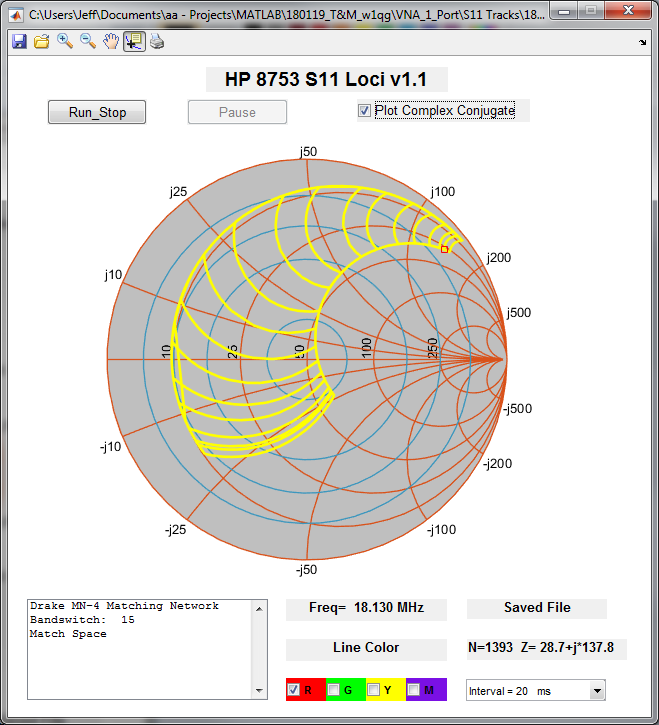
Here's the original MN-4 match-space plot made at 3.5 MHz with my VNA:


Next, I will create a model of the tuner in MATLAB to be the basis for my experiments.  But I first must ensure that the model I've created gives me results similar to the plot I made with my physical MN-4 tuner.

I will start with a model using Drake's schematic values for C5-C12 and calculating L2 and L3 to be 9.88 uH and 0.225 uH, respectively (from their dimensions and number of turns).

Matlab will calculate the resulting match-space outline using the complex-conjugate method -- placing 50 ohms at the input of the model and, while stepping through the model's two control settings, calculating the complex-conjugate of the impedance measured at the network's output.

MATLAB's resulting match-space plot of this model looks like this:


This plot is a far cry from my tuner's actual measurements!

This difference is probably due to the actual component values differing from those shown in the schematic, as well as effects caused by parasitic inductance, capacitance, and loss resistance.

Let's play with the component values (and add some network loss, too).  After jiggling them around for a bit, here's a better MATLAB match-space outline:


This new MATLAB plot is much closer to my measured plot.

And below is the circuit, with component values, that I used to generate this plot:


Caveat!  The values I selected might not accurately represent the tuner's actual component values. I chose these values because they generated a plot at 3.5 MHz similar to the one I measured. But other component values might generate a plot that is similar or even more accurate.  Do not assume the values I've chosen reflect the actual values that are in the MN-4 tuner.

OK!  Now that I've created a MATLAB model that seems to represent actual tuner performance, let's use it to run some experiments...

Let's compare the match-space with and without tuner loss (the loss model uses the resistance values from the schematic, above, while the lossless model sets all resistances to 0 ohms):


Note:  the slightly darker colors outline the match-space of the lossless network.

You can see that adding loss to the network both shrinks the match-space outline and shifts it to the right, compared to the lossless match-space outline.

But which of these two curves is closer to predicting the actual load impedances that can be matched to a 1:1 SWR?

I'll run another MATLAB experiment.  This time MATLAB will step each of the model's two tuner controls, one at a time, exactly as I would have stepped the tuning controls on a real tuner to plot the match-space outline manually.  At each incremental step, the MATLAB script will iterate through a range of load impedances, searching for an actual impedance that will give the closest match to a 1:1 SWR for those settings of the model tuner.

In other words, for every tiny change in the tuner's setting, I will search for a load impedance that transforms exactly (or almost exactly) to 50 ohms, when measured at the tuner's input port.

I've added this new plot to the figure below.


(Note: the MATLAB script uses my "jiggled" component values (that include network loss) as the Tuner's components).

The left-most outline represents actual loads that tune to 1:1 SWR, while the right-most outline represents the match-space found by terminating the input with 50 ohms and measuring the complex-conjugate of the impedance at the network's output port.

Let's remove the "lossless" plot...


Note the significant difference between the two remaining outlines.  The match-space outline representing the load impedances the tuner can actually match to a 1:1 SWR is significantly different from the match-space outline found via the "conjugate-match" method described earlier in this post.

This difference is due to loss within the network!

As a sanity check of my MATLAB model, let's see what happens to the three outlines as I reduce network loss.  The differences between the three outlines should become smaller.  To check this, I'll change all of the loss resistances to 0.2 ohms (from the values I used in the schematic, above).

Here's the plot of the three outlines with the reduced loss resistances:


Note that the three outlines are now much closer together, and they are almost coincident with the middle "lossless" outline.  If loss were reduced to zero, the three outlines would be exactly coincident.


Conclusion, the Effect of Loss on Network Match-Space Measurements:

If a two-port network has low loss, the "complex-conjugate" method (described above) can generate a fairly accurate representation of the network's match-space.  But as tuner loss increases, the loads represented by the match-space generated using the complex-conjugate method will diverge further and further from the loads that actually can be matched to a 1:1 SWR.

In other words, when measuring a network's match-space using the complex-conjugate method, be sure to also measure network power loss in order to judge how accurate your results might be.

(Note that network power-loss can be measured using the method described in the link, below:


MATLAB Scripts for Plotting VNA Data:

Dick Benson's MATLAB scripts for capturing VNA data (e.g. from an HP 8753x) and displaying it (that I use above) can be downloaded from his page in the MathWorks file exchange section:  Dick Benson MATLAB files


Antenna Tuner Blog Posts:

A quick tutorial on Smith Chart basics:
http://k6jca.blogspot.com/2015/03/a-brief-tutorial-on-smith-charts.html

Plotting Smith Chart Data in 3-D:
http://k6jca.blogspot.com/2018/09/plotting-3-d-smith-charts-with-matlab.html

The L-network:
http://k6jca.blogspot.com/2015/03/notes-on-antenna-tuners-l-network-and.html

A correction to the usual L-network design constraints:
http://k6jca.blogspot.com/2015/04/revisiting-l-network-equations-and.html

Calculating L-Network values when the components are lossy:
http://k6jca.blogspot.com/2018/09/l-networks-new-equations-for-better.html

A look at highpass T-Networks:
http://k6jca.blogspot.com/2015/04/notes-on-antenna-tuners-t-network-part-1.html

More on the W8ZR EZ-Tuner:
http://k6jca.blogspot.com/2015/05/notes-on-antenna-tuners-more-on-w8zr-ez.html  (Note that this tuner is also discussed in the highpass T-Network post).

The Elecraft KAT-500:
http://k6jca.blogspot.com/2015/05/notes-on-antenna-tuners-elecraft-kat500.html

The Nye Viking MB-V-A tuner and the Rohde Coupler:
http://k6jca.blogspot.com/2015/05/notes-on-antenna-tuners-nye-viking-mb-v.html

The Drake MN-4 Tuner:
http://k6jca.blogspot.com/2018/08/notes-on-antenna-tuners-drake-mn-4.html


Standard Caveat:

As always, I might have made a mistake in my equations, assumptions, drawings, or interpretations.  If you see anything you believe to be in error or if anything is confusing, please feel free to contact me or comment below.

And so I should add -- this information is distributed in the hope that it will be useful, but WITHOUT ANY WARRANTY; without even the implied warranty of MERCHANTABILITY or FITNESS FOR A PARTICULAR PURPOSE.

Thursday, August 16, 2018

Notes on Antenna Tuners: Drake MN-4 Matching Network

At a recent swap-meet I purchased a Drake MN-4 "Matching Network" from a friend.  This post describes notes of mine on the tuner and measurements of its performance.


MN-4 Specifications:

From the manual, the MN-4's specifications are:


Interestingly, although the manual specifies that it can match any load-impedance with a VSWR of 5:1 or less, it does not specify to what minimum SWR these loads can be tuned.  Is it 1:1 SWR?  I'll take a look at this further, below...


MN-4 Schematic:

And here is the MN-4 schematic, also from the manual:


Inside the MN-4:

I was curious what the MN-4 circuitry looked like.  After removing the black outer covers, I was surprised to find that the tuner was also well shielded:


Below is a picture of the inside of the tuner with the shield removed.  (Note that the meter is also shielded).


Let's now look at some measurements:


Tuner Performance:  Measuring a Tuner's "Match Space":

Any Antenna Tuner worth its salt should transform a wide range of impedances connected to its Output Port (i.e. its Antenna Port) to 50 ohms (i.e. 1:1 SWR at its Input (Transmitter) Port).

An obvious question is -- what is the actual range of impedances that a specific tuner can match?

It is relatively straight forward to measure these impedances (if one has a Vector Network Analyzer) and to plot them on a Smith Chart.  The resulting region of matchable impedances I call a tuner's "Match Space".

In other words, the "Match Space" is an area on a Smith Chart encompassing the range of impedances that a tuner can transform to 50 + j0 ohms at its input port.

How do we determine what these impedances are?  Do I need a box full of resistors, capacitors, and inductors to connect to the tuner's output and test each combination?

A little network theory...

Assume a two-port lossless network with an impedance of unknown value, Z(unknown), attached to its output port, and assume that the network has been "tuned" so that Z(unknown) is transformed to 50 + j0 ohms when measured at the network's input port.
(Note:  no network is truly "lossless", and I will discuss the effect of loss on these measurements at the end of this post.  But, for the moment, let us assume that the network loss is significantly less than the load's power dissipation/radiation so that the above statement is, essentially, true.)
If I then connect a 50 + j0 load to the network's input port and remove Z(unknown) from the output port, the impedance I measure at the network's output port will be the complex-conjugate of the original Z(unknown) impedance.


So, to determine a tuner's "Match Space", all I need to do is to terminate the tuner's input with 50 + j0 ohms and then, while continuously adjusting the tuner's controls, plot the complex-conjugates of the impedances I measure at the tuner's output.

An ideal task for a Vector Network Analyzer!


Equipment and Software:

To make these complex-conjugate measurements I use the following equipment and software:
  1. An HP 8753C Vector Network Analyzer (VNA) and an HP 85046A S-Parameter Test Set.
  2. An Agilent 82357B USB/GPIB Interface Module, to interface a computer to the VNA.
  3. A recent version of MATLAB, with the following toolboxes:  1) RF Toolbox, 2) Instrument Control Toolbox.
In addition, I use a MATLAB script (vna_s11_tracks.m) written by Dick Benson, W1QG, to plot the match-space on a Smith Chart.


Measurement Procedure:
  1. Connect an accurate 50 ohm reference load to the Tuner's input port (i.e. Transmitter port).
  2. Launch the MATLAB script vna_s11_tracks.m, but do not yet click its RUN_STOP button on its GUI.
  3. At the VNA set Center Frequency to the desired measurement frequency.
  4. At the VNA set Span to 0 Hz.
  5. At the VNA set Number of Points to 3 (under MENU button in the "Stimulus" button group) for the 8753C).  Default is 201 points.
  6. Perform an S11 open-short-load calibration on the end of the coax that will attach to the Tuner's output port (i.e. antenna port).  Note that the other end of this coax should already be connected to Port 1 of the S-Parameter Test Set.
  7. After calibrating, re-attach the "open" reference load to the same end of the coax that had been calibrated in step 4, above.
  8. Click on the RUN-STOP button.  (The STATUS box on the GUI should say "RUN".)
  9. Verify that a small red square outline appears exactly at the 3 o'clock position of the GUI's Smith Chart.  If it is there, then the VNA has been calibrated correctly.  If it is somewhere else on the Smith Chart, you have done something wrong.  Repeat the calibration steps, above.
  10. Click on the GUI's RUN_STOP button to stop the script.  Remove the "open" reference load from the coax and instead attach the coax to the Tuner's output port.
  11. Click RUN_STOP again and start capturing data, per either the first or second method of plotting, discussed below...
Plotting the Match Space:

For a Tuner (or other two-port network) having two variable controls, I can use the MATLAB script to plot the "Match Space" one of two ways.

The first method is the fastest, and it simply traces the outline of the match-space by sequentially holding one of the two controls fixed while rotating the other control.

In other words, say a tuner has two controls (control A and control B), this method's steps would be:
  1. Place both controls at their maximum counter-clockwise (CCW) position.
  2. With control B fixed at its counter-clockwise position and rotate control A from CCW to its maximum clockwise (CW) position.
  3. With control A now at its maximum CW position, rotate control B from its CCW position to its maximum CW position.
  4. With both controls now at their maximum CW positions, rotate control A from its CW position to its maximum CCW position.
  5. And finally, rotate control B from its CW position to its maximum CCW position.
An example of an outline-plot of a match-space, made using this method, is shown below:


(Note that Dick's MATLAB script allows the user to assign a different color to each of the steps in steps 2 through 5.  I've defined the color assignments in the comment-box at the lower left of the figure.)

An Important Caveat!  This procedure will accurately trace the outline of a Tuner's match space in most cases.  But not always!  If in doubt, then one can use a second, more time-consuming method:

Again, assuming a tuner has two controls (A and B), this second method's steps would be:
  1. Place both controls at their maximum counter-clockwise (CCW) position.
  2. With control B fixed at its maximum counter-clockwise position and rotate control A from CCW to its maximum clockwise (CW) position and back again.
  3. Rotate control B very slightly clockwise.
  4. Again, rotate control A from its CCW position to its maximum clockwise (CW) position and back again.
  5. Repeat steps 3 and 4 until control B is finally at its maximum CW position and control A has been rotated CCW and back again.
Here is an example of a plot made using this method:


In the example above (using an Icom AT-500 Tuner), I stepped one control through 14 positions, and at each step of the first control position I rotated the other control fully clockwise and then counter-clockwise back again.

This second method is much more time consuming to perform, but it can reveal information that might be missed if  one simply traced the match-space outline using the first method.  For example, below is the match-space outline (using the first technique) overlayed on the second method's plot:


Comparing the two plots, you can see that method 1 missed some of the match-space:


Also, if you examine method 2's plots, you will see that the same match-space area missed by method 1 actually has more than one unique Tuner setting for the load impedances in that region.

For example, in the figure, below, note the intersection of two different curves.  This means that the impedance represented by the Smith Chart at this intersection can be matched with two different tuner settings.


And therefore, because the entire region, above (missed by method 1) actually consists of overlapping curves, the impedances in that entire region can be each matched by two different tuner settings.

Note:  This result does not mean that, in the general case, any area missed by the method 1 (and caught by method 2) can actually be matched by multiple tuner setting.  But for this specific example, it does.


MN-4 Match-Space Measurements:

This section contains match-space plots I've made of my MN-4 tuner.  For these plots I have defined Smith Chart SWR circles representing four SWRs:  1.5:1, 3:1, 5:1, and 10:1.


80 Meter Match Space:

The MN-4 has two band-switch positions for 80 meters.  They are  80A and 80B.

First, outline-plots at 3.5 MHz for the 80A and 80B band-switch positions:


...and then, outline-plots at 4.0MHz for the 80A and 80B band-switch positions:


Note that at 3.5 MHz the Drake specification of matching loads with a VSWR of 5:1 (or less) at any impedance angle is not met, if we assume that the specification is for a match to provide a resulting SWR of 1:1.

At 4 MHz the match-space is closer to the specified 5:1 SWR, but still not quite there.


40 Meter Match Space:

An outline-plot at 7.0 MHz:


...and an outline-plot at 7.3 MHz:


Repeating the 7.3 MHz plot using method 2:


20 Meter Match Space:

The 20 meter match space outline-plot at 14.175 MHz:


15 Meter Match Space:

The 15 Meter match-space outline-plot at 21.0 MHz:


A bit of a strange plot.  How to interpret?

If I play around with the tuning controls (using plotting method 2), I discover that the match-space outline should actually encompass more impedances...


Repeating the same procedure at 21.45 MHz, the match-space outline is:


10 Meter Match Space:

Outline-plot at 28.0 MHz:


Looks pretty lousy!

Here's the match-space outline-plot at 29.7 MHz:


It's clear that on 10 meters the MN-4 does not come close to meeting the specification of matching any load with a 5:1 VSWR.


17 Meter Match Space:

I was curious how the tuner might work on the WARC bands.  So as an example, I thought I would plot the match-space for 17 meters (measured at 18.130 MHz), setting the MN-4's band-switch first to 20 meters and plotting the match-space, and then setting the band-switch to 15 meters and again plotting the match-space.

Here is an outline-plot of the 17 Meter match-space with the band-switch set to 20 Meters:


Hmmm...looks strange.  How should I interpret the big yellow circle?

Let's see what happens if I plot the match-space using the second plotting method (described earlier):


Ah-ha!  There's a big hole in the match-space!

And below is the 17 Meter match-space (plotted using the second method) with the band-switch set to 15 Meters:


In either case, the MN-4 leaves something to be desired if attempting to tune impedances on 17 meters.


Power Loss Measurements:

Measurements of internal tuner power loss versus load impedance were made using the procedure described in this blog post:


Here are my loss measurements:


Notes:

1.  The yellow rows represent load impedances that I could not tune to a 1:1 SWR.

For example, the MN-4 cannot match a 150 ohm (3:1 SWR) load on 10 meters.  The best I could do was to reduce its SWR to 1.22:1 at 29.7 MHz.

Here is the Gp plot for the 150 ohm load at 29.7 MHz:


Observe how Gp diverges from Gt when the SWR is not close to 1:1.  (Refer to http://k6jca.blogspot.com/2018/08/additional-notes-on-measuring-antenna.html for an explanation).

2.  The SWR is about 1.7:1 when the Tuner band-switch is set to DIRECT and the test frequency is on 10 meters.  The load is an excellent 50 ohm reference standard, so the SWR should ideally be 1:1.

3.  It is interesting that power-loss measured at a specific frequency is fairly constant irrespective of load impedance, even when this load impedance is 50 ohms.  This implies that the majority of the MN-4's loss is via L2 and L3, (and/or Cin), per my explanation in the diagram, below:


Continuing...

Here's a plot of S11 on 10 meters with the Reference Load of 50 ohms attached to the tuner's output port and the band-switch set to DIRECT:


That is a pretty significant SWR change to what should be, ideally, a 1:1 SWR!

Let's look at it over the range of 3.5 to 30 MHz:


Yes, it becomes worse as frequency increases.  This is probably due to the point-to-point wiring used within the tuner chassis (see photograph of the inside of the tuner, above).  But there are other suspects, too.  Let's try to eliminate them...

There are some adapters involved.  For the S11 capture, above, the VNA and load are connected to the tuner per the image, below.


Note that each port has both a PL-259 to BNC adapter and a BNC to SMA adapter.  Could these adapters be the issue?

Let's replace the tuner with an SO-239 barrel adapter:


Here is the S11 capture:


...although not perfect (i.e. 1:1 SWR), this plot is significantly better than the plot with the tuner in-line.

And finally, as a sanity check, the plot of the Reference Load, itself, attached to the coax:

Here's the configuration:


And here's its S11 capture:


Looks excellent!  But this shouldn't be surprising, because this was the configuration used for the VNA's S11 calibration.

As to why the SWR worsens in DIRECT mode, my guess is that it is due to the fairly-long point-to-point (non-coax) wiring between the SO-239 connectors and the tuner's band-switch.

You can see the interconnect wires (yellow insulation), below:


As a quick test of this theory, note that the wiring to the Dummy Load connector (the middle of the three SO-239 connectors) from the rotary switch is shorter than the wiring to the Antenna port (left-hand connector).  So, if wire length is affecting SWR, there should be less effect if I measure the SWR to the tuner's Dummy Load port.

Here's the Reference Load connection:


And here's the S11 capture.


Note the improvement in SWR.  Not an earth-shattering improvement, but I believe it supports my point.

So, if I were going to attempt to improve its performance, the first thing I would try is replacing those yellow wires (see photo of the interior of the tuner, above) with coax.


Effect of Network Loss on Match-Space Measurements:

As I mentioned earlier in this post, the Match-Space can be found by terminating the network's input port with 50 ohms and measuring the transformed-impedance at the network's output port.  This impedance represents the complex-conjugate of a load impedance that, when attached to the network's output port, will appear as 50 ohms at the network's input port.

But this relationship is only true if the network is lossless.  If the network has loss, there will be error introduced into this complex-conjugate impedance measurement.

Let's look at this error with respect to my MN-4 measurements.

When I measured the tuner's power loss with different loads, I also measured the complex-conjugate of the impedance seen at the tuner's output port when its input was terminated with 50 ohms.

If there were no loss, the impedance I measure should be the same as the original load impedance I had used to make the power-loss measurement.  For example, if I had tuned the tuner to match a load of 150 ohms, then, when I removed the load and attached 50 ohms to the tuner's input port, the measured impedance at the output port should also be 150 ohms.

But I measure a different value.  And it turns out that the greater the network power loss, the greater will be the difference between the actual load value (used for power-loss measurements) and the load value calculated via the complex-conjugate method.

Here's a table containing both the network loss for different loads and the impedance measured at the output port using the complex-conjugate method when the input was terminated with 50 ohms:


(Note the yellow rows -- these are load impedances that I could not tune to 1:1 SWR).

There's a significant difference between the complex-conjugate measurement and the actual load value.  And as you can see, the greater the loss, the greater the error.

Let's explore further, using MATLAB...


Using MATLAB to Examine Loss Effects on Match Space Plots:

How does network loss affect the Drake MN-4's match-space at 3.5 MHz?

Here's the original MN-4 match-space plot made with my VNA:


Next, I will create a model of the tuner in MATLAB to be the basis for my experiments.  But I first must ensure that the model I've created gives me results similar to the plot I made with my physical MN-4 tuner.

Matlab will calculate the resulting match-space outline using the complex-conjugate method -- placing 50 ohms at the input of the model and, while stepping through the model's two control settings, calculating the complex-conjugate of the impedance measured at the network's output.

MATLAB's resulting match-space plot of this model looks like this:


This plot is a far cry from my actual measurements!

This difference is probably due to the actual component values differing from those shown in the schematic, as well as effects caused by parasitic inductance, capacitance, and loss resistance.

Let's play around with the component values (and add some network loss, too).  Here's a new MATLAB match-space outline:


This new MATLAB plot is much closer to my measured plot.

And below is the circuit, with component values, that I used to generate this plot:


Caveat!  The values I selected might not accurately represent the tuner's actual component values.  I chose these values because they generated a plot similar to the one I measured.  But other component values might generate a plot that is similar or even more accurate.  Do not assume the values I've chosen reflect the actual values that are in the MN-4 tuner.

OK!  Now that I've created a MATLAB model that seems to represent (fairly closely) tuner performance, let's use it to run some experiments...

Let's use MATLAB to compare the match-space with and without tuner loss (i.e. set all resistances to 0 ohms for the lossless network), using the complex-conjugate technique to calculate the impedances that are matched:


Note:  the slightly darker colors outline the match-space of the lossless network.

You can see that adding loss to the modeled network and performing the complex-conjugate calculation with this loss included shifts the match-space outline to the right, compared to the calculated lossless match-space outline.

But which of these two curves is closer to predicting the actual load impedances that can be matched to a 1:1 SWR?

I'll run another MATLAB experiment.  This time MATLAB will step each of the model's two tuner controls, one at a time, exactly as I would have stepped the tuning controls on a real tuner to plot the match-space outline manually.  At each incremental step, the MATLAB script will iterate through a range of load impedances, searching for an actual impedance that will give the closest match to a 1:1 SWR for those settings of the model tuner.

In other words, for every tiny change in the tuner's setting, I will search for a load impedance that transforms exactly (or almost exactly) to 50 ohms, when measured at the tuner's input port.

I've added this new plot to the figure below.


This new plot is the left-most plot, and it represents the outline of the impedances that the modeled tuner actually tunes to a 1:1 SWR.

The middle plot represents the match-space calculated via the complex-conjugate method with no network loss, while the right-hand plot represents the match-space calculated via the complex-conjugate method with network loss.

There's a large difference between the left-hand and the right-hand plot.  Clearly including loss in the tuner model when calculating the match-space via the complex-conjugate method is not the approach to take.  Better to assume that the network is lossless (at least in the case of the Drake MN-4).

As a sanity check of my MATLAB model, let's see what happens to the three outlines as I reduce network loss.  The differences between the three outlines should become smaller.  To check this, I'll change all of the loss resistances to 0.2 ohms (from the values I used in the schematic, above).

Here's the plot of the three outlines with the reduced loss resistances:


Note that the three outlines are now much closer together, and they are almost coincident with the middle "lossless" outline.  If loss were reduced to zero, the three outlines would be exactly coincident.


Conclusion, the Effect of Loss on Network Match-Space Measurements:

If a two-port network has low loss, the "complex-conjugate" method (described above) can generate a fairly accurate representation of the network's match-space.  But as tuner loss increases, the loads represented by the match-space generated using the complex-conjugate method will diverge further and further from the loads that actually can be matched to a 1:1 SWR.

In other words, when measuring a network's match-space using the complex-conjugate method, be sure to also measure network power loss in order to judge how accurate your results might be.


MATLAB Scripts for Plotting VNA Data:

Dick Benson's MATLAB scripts for capturing VNA data (e.g. from an HP 8753x) and displaying it (that I use above) can be downloaded from his page in the MathWorks file exchange section:  Dick Benson MATLAB files


Antenna Tuner Blog Posts:

A quick tutorial on Smith Chart basics:
http://k6jca.blogspot.com/2015/03/a-brief-tutorial-on-smith-charts.html

Plotting Smith Chart Data in 3-D:
http://k6jca.blogspot.com/2018/09/plotting-3-d-smith-charts-with-matlab.html

The L-network:
http://k6jca.blogspot.com/2015/03/notes-on-antenna-tuners-l-network-and.html

A correction to the usual L-network design constraints:
http://k6jca.blogspot.com/2015/04/revisiting-l-network-equations-and.html

Calculating L-Network values when the components are lossy:
http://k6jca.blogspot.com/2018/09/l-networks-new-equations-for-better.html

A look at highpass T-Networks:
http://k6jca.blogspot.com/2015/04/notes-on-antenna-tuners-t-network-part-1.html

More on the W8ZR EZ-Tuner:
http://k6jca.blogspot.com/2015/05/notes-on-antenna-tuners-more-on-w8zr-ez.html  (Note that this tuner is also discussed in the highpass T-Network post).

The Elecraft KAT-500:
http://k6jca.blogspot.com/2015/05/notes-on-antenna-tuners-elecraft-kat500.html

The Nye Viking MB-V-A tuner and the Rohde Coupler:
http://k6jca.blogspot.com/2015/05/notes-on-antenna-tuners-nye-viking-mb-v.html

The Drake MN-4 Tuner:
http://k6jca.blogspot.com/2018/08/notes-on-antenna-tuners-drake-mn-4.html


Standard Caveat:

As always, I might have made a mistake in my equations, assumptions, drawings, or interpretations.  If you see anything you believe to be in error or if anything is confusing, please feel free to contact me or comment below.

And so I should add -- this information is distributed in the hope that it will be useful, but WITHOUT ANY WARRANTY; without even the implied warranty of MERCHANTABILITY or FITNESS FOR A PARTICULAR PURPOSE.