The Quarter-wave Transformer: Transient and Steady-State Reflections

This post is the second post of two analyzing transient and steady-state reflections in systems with transmission lines and impedance matching devices.

This analysis is done using the system's Impulse Response and convolving that with a Stimulus that is bounded in time (that is, the stimulus has a defined start time and a defined stop time).

This method of using the Convolution Integral allows us to examine both the system's transient response (when the stimulus switches from absent to present or from present to absent) and  its steady-state response.  For more background on this technique, please refer to my first post in this series:  Antenna Tuners: Transient and Steady-state Analysis.

The Quarter-wave Transformer:

The quarter-wave impedance transformer is a two-port impedance-matching device consisting of a quarter wavelength of transmission line whose characteristic impedance is the square-root of the product of the impedances attached at its two ports.

For example, in the drawing above, Transmission Line 2 will match the load (Rload) to the characteristic impedance of Transmission Line 1 (Za) if Transmission Line 2's characteristic impedance (Zb) is the square-root of the product of Za and Rload:

Zb = (Za*Rload)^0.5

Calculating the System's Impulse Response:

To analyze the transient-state of the reflections within the matching system using the Convolution Integral, I first need to calculate the system's impulse response (i.e. its response to a single impulse).

To simplify the analysis, I'll assume that the transmission lines are lossless and behave like perfect delay lines.  Also, I will assume that the Source is matched to Transmission Line 1.

Therefore, an impulse traveling on one transmission line, when it arrives at the second transmission line of a different impedance, will be divided into two parts at the impedance discontinuity.  One part is reflected backwards in the opposite direction of travel and the other part continues forward.  Their amplitudes as they travel along the transmission lines will only be a function of the various Reflection and Transmission Coefficients within the antenna system and not due to transmission line loss.

The Reflection and Transmission Coefficients that a single impulse sees as it travels through the antenna system are solely the function of the impedances immediately at either side of an impedance discontinuity, and they are calculated using the standard formulas:

R = (Zb - Za)/(Zb + Za)

T = 2Zb/(Zb + Za)

where Zb is the impedance that the impulse is traveling to, and Za the impedance it is traveling from.

The drawing below shows the calculated Reflection and Transmission Coefficients at each impedance discontinuity, assuming the load is 200 ohms, the characteristic impedance of Transmission Line 1 is 50 ohms, and the characteristic impedance of the Quarter-wave Transformer (Transmission Line 2) is 100 ohms:

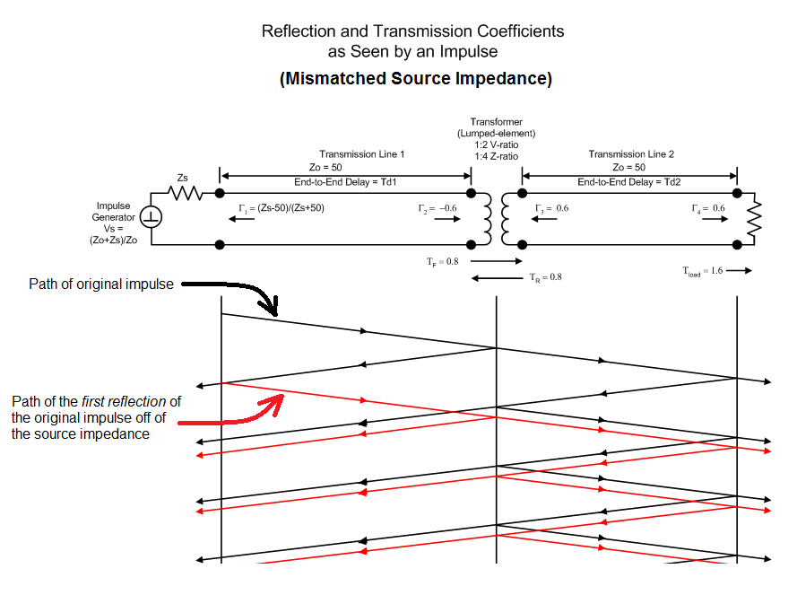
If I shoot a single impulse from the source into Transmission Line 1, it will move from left to right until it reaches the discontinuity at Transmission Line 2.  At that point, a portion of the impulse will continue onwards, towards the load, while a second portion is reflected back to the source.  

(Note that I've defined the source to be matched to Transmission Line 1, so there is no re-reflection back towards the load when this part of the impulse arrives back at the source).

The first portion, when it reaches the load, will again see an impedance discontinuity and it will again be divided into two parts.  One part is dissipated by the load's resistance, and the other part is reflected back towards Transmission Line 1.

When this reflection from the load reaches Transmission Line 1, it is again divided into to parts.  One part reflects back to the load, and one part passes through the impedance discontinuity and continues back to the source.

And thus it goes -- there will be an infinite number of reflections and re-reflections on Transmission Line 2.

Below is a diagram showing the amplitudes of the impulse (in terms of Reflection and Transmission coefficients) as it is divided into two parts whenever it reaches an impedance discontinuity:

For example, let Vi(t) be a single impulse in time.  Let's define its arrival (from the source) at the impedance discontinuity between Transmission Line 1 and Transmission Line 2 to be at time t = 0.  

From the lattice diagram above I can calculate impulse responses for Vr1, Vf2, Vr2, and Vld.  

For example, Vr1 (the voltage seen at the interface between the two transmission line that is traveling back towards the source) can be expressed mathematically as an infinite series.  It is the terms in this series that define the impulse response of Vr1:

Here is the Impulse Response of Vr1 (calculated with MATLAB):

You can see that the higher terms of the series (which is infinite in length) quickly become imperceptible compared to the first few terms.

Similar infinite series can be written using the terms in the Lattice Diagram for the voltages Vf2, Vr2, and Vld, and from these series the Impulse Response of each voltage can be calculated.

Convolving the  System's Impulse Response with a Sinusoidal Stimulus:

I can take the calculated impulse responses of Vr1, Vf2, Vr2, and Vld and, using the Convolution Integral, calculate their output waveforms for any input stimulus waveform.

But because the quarter-wave transformer is an impedance-matching device defined for use at a single frequency where its length is a quarter-wavelength of the stimulus signal, the stimulus I will use will be a sine wave.  (A quarter wave-length thus represents one-quarter cycle of the sine wave).

In steady-state (with a sinusoidal drive), the signal from the source arriving at the interface of the two transmission lines will be either in-phase or 180 degrees out-of-phase with the reflections arriving back from the load, depending upon how many up-and-back trips a reflection has made (they will be out-of-phase if the number of trips is odd, in-phase if the number of trips is even). 

Therefore, we can express Vr2 as the following infinite series.  Note that the phase of the arriving reflection flips between 0 and 180 degrees with each term, depending upon if the number of round-trips it has taken on the second transmission line is even or odd..

The final equation in the figure, above, contains an infinite geometric series that converges to a value.  We can calculate this value using the formula below for solving infinite geometric series:

Solving for Vr1's infinite series, we find the following: 

Using the same technique, we can also calculate the steady-state equations for Vf2, Vr2, and Vld, which are:

Given a sine-wave signal Vi(t) of amplitude equal to 1, the steady-solutions for these equations are shown at the bottom of the lattice diagram, below:

(Note:  we can also use the earlier equation for "Apparent Γ₂" to find the equation that calculates the required characteristic impedance of Transmission Line 2, given the load impedance and the characteristic impedance of Transmission Line 1, that will result in an "Apparent Γ₂" equal to 0.  See: Multiple Reflections and the Quarter-wave Transformer.)

Convolution Results:

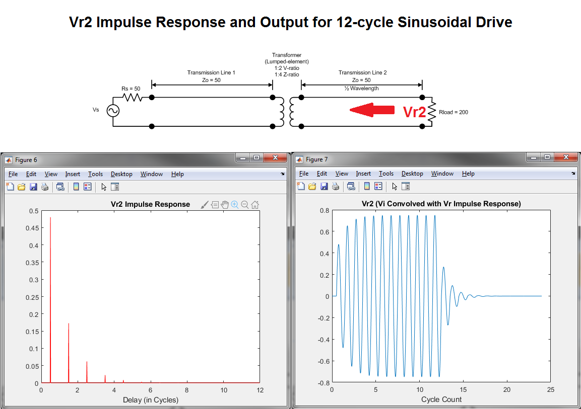
I've used MATLAB to first calculate the impulse responses of Vr1, Vf1, Vr2, and Vld, and then to convolve these impulse responses with the sinusoidal stimulus.  I've plotted the results, below.

Below is the stimulus, Vi(t).  It is present for 12 cycles and otherwise off:

Below are the MATLAB plots of Vr1's impulse response and resulting output when convolved with the stimulus.  You can see the non-zero transient response at the start and finish of the sine-wave.  And in steady state Vr1 goes to 0. 

For convenience, I've plotted the stimulus and the Vr1 output together, below:

Below are Vf2's impulse response and resulting output when it is convolved with the stimulus.  

Below are Vr2's impulse response and resulting output when it is convolved with the stimulus. 

And finally, below are Vld's impulse response and resulting output when it is convolved with the stimulus. 

Again, for convenience, I've plotted the stimulus and the Vld output together, below:

You can see the quarter-cycle delay between the stimulus and Vld in the plot, above.

The Re-reflection of Vr2:

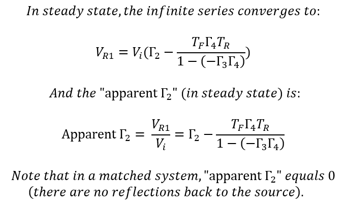
In steady-state it is clear that some portion of the Vr2 voltage continues through the discontinuity towards the source.  This is why the wave heading back to the source (Vr1) goes to 0 in steady-state (when load is matched to Transmission Line 1) -- this transmitted part of Vr2 cancels the part of Vi that is reflected by the transformer's input discontinuity.

But some part of Vr2 is reflected back to the load.  How much?  And (assuming that the quarter-wave line is matching load to Transmission Line 1) does  Γ₃ change in steady-state (in a fashion similar to how Γ₂ changes to to an "apparent"  Γ₂ of 0)?

We can calculate the steady-state Γ₃ using the same steady-state equations for Vf2 and Vr2 that were derived earlier.

First, let's call this reflection of Vr2 off of the quarter-wave transformer's "input" impedance discontinuity "Vr2Re_Reflected".  This is the portion of Vr2 that is re-reflected back to the load by the impedance discontinuity (the other part continues through the discontinuity to the source)

This re-reflected voltage sums with the forward voltage from the source that is passing through the input discontinuity towards the load.  In other words, Vf2 = Vi(0°)Tf + Vr2Re_Reflected.

Therefore Vr2Re_Reflected = Vf2 - Vi(0°)Tf , and the "apparent" Γ₃ should therefore be the ratio of Vr2Re_Reflected to Vr2.

Using these relationships and recognizing that Vr2 is 180 degrees out of phase with Vi when Vr2 arrives back at the input to the quarter-wave transformer, we can derive the "apparent" Γ₃ as follows:

Therefore, the steady-state "apparent" Γ₃ is the same as the original Γ₃ calculated for a single impulse on the line.

Given a sinusoidal source driving a 1 volt signal onto the first transmission line, the following illustration summarizes the steady-state voltages in the system.  Note that the blue line represents the signal that is just arriving from the source, while the green lines represent the reflections and re-reflections of previous signals from the source.

Conclusions:

1.  As with any other linear system, the Convolution Integral allows us to calculate the time-domain transient and steady-state responses of the system to a stimulus.

2.  Given a sine-wave stimulus that is bounded in time, there are reflections back to the source during the system's transient states.  These reflections decay to 0 in the steady-state, resulting in an "apparent" Γ₂ of 0.

3.  In the steady-state, Vf2 is a combination of the forward signal arriving from the source (scaled by the Transmission factor of the impedance discontinuity between the two transmission lines) and the re-reflection by Γ₃, at the impedance discontinuity between the two transmission lines, of the backwards traveling Vr2 wave (from the load).  The amplitude of this re-reflection equals Vr2 * |Γ₃|.

4.  Assuming that the quarter-wave transformer is matching the load to Transmission Line 1's characteristic impedance, in steady-state Γ₃ remains unchanged from the value calculated for an impulse response, and Γ₃ is independent of the source impedance.  In other words, because there are no signals sent back to the source in steady-state, it does not matter what the source impedance is because there is no signal to be reflected back by a possible source mismatch.

Additional Notes:

1.  Quarter-Wave Transformer Input Impedance:

Although not obvious from the Lattice Diagram, above, the Input Impedance of a Quarter-Wave Transformer is independent of the impedance of the "left-hand" transmission line (or lumped-element source impedance, if there is no transmission line) attached to its input port.

In other words, the Transformer's Input Impedance is only a function of the characteristic impedance Zo of the quarter-wave line and the load impedance attached to the output of the Transformer.

Regarding the diagram, above, this would mean that if the characteristic impedance of the left-hand transmission line (Za) was not 50 ohms, there would be reflections from the input of the transformer back towards the source that do not go to zero in steady-state.

Also, the transient voltage levels of the waves on the transformer's transmission line (Vf1, Vf2, and Vr2) would be different.  

But despite these differences, in steady state the sum of Vf1 and Vf2 (i.e. the overall Vf on the transformer's transmission line moving towards the load), and the level of Vr2 (moving from the load back), would remain unchanged.

And if a "lumped-element" directional coupler (i.e. SWR meter), referenced to 50 ohms, were placed on Transmission Line 1 at the input to the transformer, it would read an SWR of 1:1, irrespective of the Transmission Line 1's characteristic impedance.

Other Transmission-Line Posts:

http://k6jca.blogspot.com/2021/02/antenna-tuners-transient-and-steady.html.  This post analyzes the transient and steady-state response of a simple impedance matching system consisting of a wide-band transformer.  I calculate the system's impulse response and find the time-domain response by convolving this impulse-response with a stimulus signal.

http://k6jca.blogspot.com/2021/02/the-quarter-wave-transformer-transient.html.   This post analyzes the transient and steady-state response of a Quarter-Wave Transformer impedance matching device.  I calculate the system's impulse response and find the time-domain response by convolving this impulse-response with a stimulus signal.

http://k6jca.blogspot.com/2021/03/useful-swr-voltage-and-power-equations.html.  This post lists (in an easily accessible location that I can find!) some equations that I find useful

http://k6jca.blogspot.com/2021/05/antenna-tuners-lumped-element-tuner.html.  This post analyzes the transient and steady-state reflections of a lumped-element tuner (i.e. the common antenna tuner).  I describe a method for making these calculations, and I note that the tuner's match is independent of the source impedance.

http://k6jca.blogspot.com/2021/05/lc-network-reflection-and-transmission.html.  This post describes how to calculate the "Transmission Coefficient" through a lumped-element network (and also its Reflection Coefficient) if it were inserted into a transmission line.  

http://k6jca.blogspot.com/2021/09/does-source-impedance-affect-swr.html.  This post shows mathematically that source impedance does not affect a transmission line's SWR.  This conclusion is then demonstrated with Simulink simulations.

https://k6jca.blogspot.com/2021/10/revisiting-maxwells-tutorial-concerning.html  This posts revisits Walt Maxwell's 2004  QEX rebuttal of Steven Best's 2001 3-part series on Transmission Line Wave Mechanics.  In this post I show simulation results which support Best's conclusions.

Standard Caveat:

I might have made a mistake in my designs, equations, schematics, models, etc. If anything looks confusing or wrong to you, please feel free to comment below or send me an email.

Also, I will note:

This design and any associated information is distributed in the hope that it will be useful, but WITHOUT ANY WARRANTY; without even the implied warranty of MERCHANTABILITY or FITNESS FOR A PARTICULAR PURPOSE.

Antenna Tuners: Transient and Steady-State Reflections

Summary

This blogpost uses the Convolution Integral to examine the transient and steady-state values of forward and reflected waves in a simple "thought-experiment" model of an antenna system consisting a mismatched load, a transmission line, an impedance matching device, a second transmission line, and  a source.

Transient and Steady-state responses are derived by convolving (using the Convolution Integral) a Stimulus with the antenna system's calculated Impulse Responses at various points of the system.

This convolution integral technique does not replace the traditional "frequency domain" method of calculating reflections.  Calculations using the latter technique are much easier to perform, but they do not allow for transient analysis, and that is the virtue of the convolution integral -- it lets us examine the system in its transient state, and from that analysis gain a better understanding of the reflection and transmission mechanisms underlying the measured reflected and transmitted steady-state wave-forms.

If we define a "matched system" as being a system in which a matching device matches an unmatched load to a transmission line connected to the source, then the analysis of the model shows that, as the "matched system" transits through its transient state to steady-state, the Reflection Coefficient looking into the input of the matching device (looking from the direction of the source) goes from a non-zero value to 0.  

That is, in the transient state there are reflections back to the source, but these reflections go to 0 in the steady-state.

However (again in the matched system), the model's steady-state Reflection Coefficient looking backwards from the load into the matching device's output port remains unchanged (from the value calculated for the impulse response), irrespective of source impedance, even in steady-state.

For a similar analysis of a quarter-wave impedance transformer, go here:  Quarter-wave Transformer: Transient and Steady-state.

Antenna Tuners:  Transient and Steady-state Reflections

I've long agreed with the "Theory of Multiple Reflections" as an explanation of the wave-phenomena that occurs on a transmission line between a mismatched load at one end and an impedance matching device at the other end (or within an impedance matching device, should that device be a distributed-element device such as a quarter-wave matching transformer, rather than a lumped-element device, i.e. Multiple-reflections and the Quarter-wave Transformer).

In the example shown below, there are steady-state Forward and Reflected waves on Transmission Line 2 (between the mismatched antenna and the matching network).  But, because of the impedance transformation provided by the matching network, no reflections return to the transmitter. 

The "Theory of Multiple Reflections" explains how these reflected and transmitted waves build from zero-state (when the transmitted signal goes from being absent to being present), and it reveals that, at startup, a portion of the initial forward wave from the transmitter is actually reflected back to the transmitter by the Matching Network even though, when steady-state is reached, this reflected signal becomes zero.

 In this blog post I will look more closely at how the forward and reflected waves behave both during their transient states (at signal startup or shutdown) and during their steady-states.

Convolution integration can be daunting if a system's impulse response is complex.  So, to keep my example's impulse response simple, I have created a model of ideal components consisting of:

• A 200 ohm resistive load.
• A half-wavelength length of "ideal" transmission line (no loss, infinite bandwidth, velocity factor equal to 1) between the load and the output port of a matching network.  (Being a half-wavelength long, the steady-state impedance looking into the "input" of this transmission line equals the impedance attached to the far end of this transmission line.  In this example, the steady-state impedance looking into this transmission line is the load resistance 200 ohms, irrespective of transmission line Zo (it just needs to be a half-wavelength long), but I will assume a Zo of 50 ohms.
• A matching network consisting of a transformer whose turns ratio (N) is 1:2.  Therefore the voltage ratio is 1:2 (in to out) and the impedance ratio is 1:4.  A 200 ohm load connected to the output of this transformer looks like 50 ohms at the transformer's input.  (The transformer is also assumed to be ideal).
• A length of  "ideal"50-ohm transmission line between the source and the transformer's input port.
• And an "ideal" Thevenin-equivalent source whose source resistance is 50 ohms (so that, if any reflections do arrive back at the source, they are absorbed and not re-reflected).

Here's the model:

Reflection and Transmission Coefficients:

Both the transformer and the load have a set of Reflection and Transmission coefficients.   These are shown in the two illustrations, below.   Note that I've derived equations for the general case and calculated values defined for this particular model (e.g. 200 ohm load, etc.)

For two-port devices such as the transformer, I sometimes find it useful to imagine its ports attached to transmission lines that are infinitely long when calculating its Reflection and Transmission coefficients (to remove the effects of any upstream or downstream impedance discontinuities).  

But if calculating these coefficients for the purposes of deriving an impulse response, we only need to use the impedances immediately on either side of a discontinuity (that is, the impedances locally, from a lumped-element perspective) at either port of the two-port device).  These are the impedances seen by a single impulse immediately upon its arrival at the two-port device.

It is important to note:  calculated for an impulse, the Transformer's Reflection and Transmission Coefficients do not depend upon the source or load impedances that might be at the ends of  transmission lines attached to these ports.

Below is the model with these Reflection and Transmission coefficients added:

Convolution:

The "Theory of Multiple Reflections" would appear to be an esoteric theory, but at its heart it is just the convolution of a stimulus waveform (any type of waveform) with the antenna system's impulse response.  And as such, it allows us to look at the time-domain transient and steady-state responses of this system to a stimulus.

Here is a definition of the convolution integral (from my college textbook):

(From Basic Circuit Theory, Desoer and Kuh, 1969, McGraw-Hill Book Co.)

With this integral, we can calculate both the transient and steady-state responses of a system (whose "impulse response" has first been characterized) to any input signal.

Electrical Engineers will be familiar with the concept of convolution.  It is taught in basic circuit-theory courses, and it is based upon the concept that any signal can be represented by an infinite number of consecutive, independent, infinitely narrow impulses.  (The amplitude of each impulse, at a particular time T, is equal to the original signal's amplitude at that same time.)

A system's time-domain response to a stimulus signal is then simply the integration of each individual impulse (representing the stimulus) with the system's impulse response.

Anyone who has designed a digital Finite Impulse Response (FIR) filter has, in fact, implemented a convolution integral whether they know it or not.  The values of the FIR filter's coefficients are simply the values of the impulse response (in time) of a filter with the desired frequency characteristics.  The FIR architecture performs the convolution integral of the input signal with this impulse response, and the output is therefore a time-domain representation of the input signal, now filtered.

For those interested in learning more about the Convolution Integral, there is much more on the web regarding this topic (for example, see: Analog Devices: Convolution).

Characterizing the System's Impulse Response:

I've chosen my model's components to simplify the calculation of its impulse response.  Ideal components that are wide bandwidth and lossless makes this process straight-forward.  For example, the half-wavelength of transmission line can be thought of as an ideal delay-line whose delay equals half the period of a sine-wave cycle.  And the transformer, being ideal, will change the amplitude of an impulse but not its shape.

So, to derive the system's impulse response I simply "drive" a single impulse (of amplitude "1") onto the first transmission line and calculate what happens as it moves through my model.

At each impedance discontinuity the impulse will be divided into two parts -- one part continues on, while the other part is reflected backwards.  The amplitudes of these two parts  are determined by the  Reflection and Transmission coefficients defined for that discontinuity (and they are such that energy is conserved).  

The diagram below illustrates this concept of transmission and reflection:

(The image above can be a bit hard to read, so below are the same reflections spread out across three drawings):

Because I've defined my system to only have loss in the load and source resistances, these reflections of the single impulse, although they continue essentially forever, becoming smaller and smaller over time.

Note, too, that after the single impulse is generated by the source, the source's voltage is 0.  Therefore, the voltage source can be replaced by a short circuit for all future calculations (as shown in the diagram, above), leaving only the source resistance connected directly to ground.

The drawing below is a Lattice Diagram (also known as Lattice Chart) that shows the time-delays and the values of the reflected and transmitted voltages in terms of each of the system's Reflection and Transmission Coefficients.

If we sum these signals over time, we get an impulse response.  For example, I've shown the impulse response for Vr2, below:

And Vr1 is an infinite series:

(Note that time is defined such that  the impulse arrives at the discontinuity between the two transmission lines at time t = 0).

Now, let's imagine that Vi is a periodic waveform (such as a sine wave) whose period equals 2*Td2 (i.e. the signal's period is twice the time delay of the second transmission line (defined to be ideal with a velocity factor equal to 1)).  In other words, Transmission Line 2 is a half-wavelength long.

If we convolve this periodic signal with one of the calculated impulse responses for this model (i.e. the impulse response for Vr1, Vf2, Vr2, or Vld), at each instant that we perform an integration, Vi will be constant because we are looking at a string of samples that are each one cycle (360°) apart.

For example, let's say we take a snapshot of all of the reflections in the system when the incoming sine is at 0 degrees.  All of the other terms will also have 0 degrees, too, because they are all 360 degrees (one wavelength) apart.  I've shown this in the equation, below:

Therefore, although the reflections continue indefinitely, they equal a geometric series that, in fact, converge to steady-state values (these steady-state values are the values we measure on our Power and SWR meters).

We can use the following equation to calculate the values to which these series converge:

In the case of my simple model, the series and the calculated-values to which they converge are shown below:

Note that Vi is constant solely because the period of the waveform is the same as the time it takes to make a round-trip journey on Transmission Line 2.  If we were to take a random snapshot of all of the reflections in the system at one instant in time, the angle of the sines that are summed in the series would all equal.  If either of these conditions did not exist, Vi would not be constant and we could not reduce the infinite series to the steady-state equations, above.

Calculating Transient and Steady-state Responses via the Convolution Integral:

To demonstrate transient and steady-state responses, I will define a stimulus that is limited in time: a 12-cycle sinusoidal signal.  The stimulus is 0 before the start of the cycles and 0 following the completion of the 12 cycles.

The delay of the second transmission line (between transformer and load) is defined to be half the period of a single cycle of the sine-wave, above (i.e. it is a half-wavelength of line).

I have used MATLAB to calculate both the impulse-response coefficients and the convolution of this 12-cycle sinusoidal signal with the impulse responses as seen at different points in the model.  These will be shown, below

Impulse-response and Convolution Results: Reflected Signal from the Transformer's Input:

Below is the impulse-response (left) and the resulting output response (right) of the voltage reflected from the transformer's input (Vr1), given the 12-cycle sinusoidal "Vi" driving signal defined above.

(Note that the delay of the first impulse is 0, which means that I'm defining Vr1 and Vi as referenced, in time, to when Vi arrives at the Transformer's input.

Note, too, that there are significant reflections back to the source during the system's transient states.  But these reflections decay to a steady-state value of essentially zero after only a few cycles.

Here's a plot showing both the stimulus and the Vr1 signal (stimulus convolved with Vr1 impulse response), superimposed:

Impulse-response and Convolution Results: Forward Signal from the Transformer's Output:

Similarly, the plots below show the impulse-response and output response for Vf2, the voltage at the Transformer's output traveling the load.

Impulse-response and Convolution Results: Reflected Signal from the Load:

Below is the impulse-response and the output response for the voltage reflected from the load (and measured at the load -- thus the first impulse-response coefficient is delayed from T = 0 by one-half cycle of Vi.  In other words, it is delayed by the length of the half-wavelength of transmission line.

Impulse-response and Convolution Results: Voltage across the Load:

And finally, below is the impulse response and the output response across the load.  This is the voltage that is dissipated as power by the load.

Below is a plot showing both the stimulus and the Vload signal (stimulus convolved with Vload impulse response), superimposed: 

(You can see the half-cycle of delay created by the half-wavelength length of the second transmission line.)

Summary of the Steady-state Response:

The drawing below summarizes the steady-state of the model when stimulated with a 12-cycle sinusoidal drive signal.

(= Vi(0°)*T_F) 

In steady-state, the part of the driven signal that reflects from the input of the transformer back to the source (and that is occurring now) is 180 degrees out of phase with the reflections from the load (Vr) that are passing through the transformer from its output port to its input (i.e. this "now" reflection has a minus sign, the other reflections passing through the transformer have a positive sign).  In the steady-state they cancel (0.6 - 0.6 = 0 volts), and no reflection returns back to the source.

Because of this voltage cancellation, overall there is no reflected wave from the transformer's input in steady-state.  And thus the apparent Reflection Coefficient at the transformer's input is 0 in steady-state.

And this is my first point: if we define a "matched system" as being a system in which a matching device matches an unmatched load to a transmission line connected to the source, then this model's analysis shows that as it transitions through its transient state to steady-state, the model's Reflection Coefficient looking into the input of the matching device (looking from the direction of the source) goes from a non-zero value to 0.  

That is, in the transient state there are reflections back to the source, but these reflections go to 0 in the steady-state.

However, even though it appears that no signal is reflected from the transformer's input in steady-state, the signal transmitted through the transformer (from input to output) is still the amplitude of the driven signal at the transformer's input (1.0 volt) times the transformer's Forward Transmission Coefficient T_F (= 0.8).  This value equals Vi(0°)*T_F   =  1V * 0.8 = 0.8V

Next, let's look at Vr2 and Vf2 on Transmission Line 2, between the transformer's output and the load:

First, we know that (by solving the infinite series), in steady state Vf2 converges to be 1.25 volts.

Note that Vf2, traveling from the transformer's output towards the load, consists of two voltages (both traveling in the same direction and in-phase) summed together.  These voltages are the portion of the generator's "now" signal that has just passed through the transformer towards the load ( = Vi(0°)*T_F   =  1V * 0.8 = 0.8V, that is, the blue line pointing right in the figure above) and the portion of Vr2 that is re-reflected by the mismatch looking into the transformer's output port (the green line pointing right in the figure above).

The re-reflection of Vr2 occurs when Vr2, traveling from the load back to the transformer's output port, sees a Reflection Coefficient of 0.6 (Γ₃) at the Transformer's output port.  Part of Vr2 re-reflects back towards the load and the remaining part continues through the transformer towards the source (as discussed in the paragraphs above).  Let's label the part that is re-reflected back towards the load as "Vr2(re-reflected)".

From the solution of our infinite series we know that Vr2's steady state value is 0.75 volts (which is the same as Vf2 multiplied by the load's Reflection Coefficient (0.75 = 1.25 * 0.6)). 

So, Vr2(re-reflected) that is now traveling towards the load equals 0.75 volts times the transformer output's Reflection Coefficient (Γ₃) of  0.6 (i.e. 0.45 volts ).  This forward-traveling re-reflected voltage is in phase with the "now" forward-traveling 0.8V that has just passed through the transformer.  These two voltages sum, and because they are in phase, the total Vf2 on the half-wavelength of Transmission Line 2 is therefore 1.25 volts (i.e. 0.8 + 0.45 volts).

(The portion of Vf2 that is not reflected by the load continues to the load  (i.e. Vf2 times the load's Transmission Coefficient, or 1.25 * 1.6) where it is dissipated as power (i.e. radiated).)

And this is my second point:  In the matched system represented by this model, the steady-state Reflection Coefficient looking backwards from the load into the matching device's output port remains unchanged from our original calculation of  Γ₃ that was based upon "local" impedances connected to the ports of the matching device (as seen be a single impulse), irrespective of source impedance, even in steady-state.

This latter conclusion should be intuitively obvious.  If, in the steady-state, there are no reflections heading back to the source (because in steady-state it looks likes a matched system), then it does not matter what the source impedance is.  With no signal coming towards it, the source is not reflecting anything back to the matching device's input, and so the source impedance has no effect on the Reflection Coefficient seen looking into the matching device's output.

Below is the same diagram of forward and reflected voltages, but for a transmitted power of 100 watts delivered to the load.

A quick check...

These relationships between Vr2 and Vf2 can be shown mathematically using the equations derived for  the infinite series, developed earlier.  Unsurprisingly, the results equal the Reflection Coefficients at load and at the transformer's output port:

First, for Vr2/Vf2:

The equation calculating the re-reflection of Vr2 at the transformer's output is shown below.  Note that this is the voltage of the forward green line in the drawing, above.  Because this re-reflection is now part of Vf2 (it is moving towards the load), we can calculate it by first subtracting out the forward blue line's voltage from the overall Vf2 equation (the voltage on the blue line is in phase with the voltage on the green line).  This will leave the re-reflected Vr2 (the forward green line's voltage) as the result.  In other words:

Important note!  Using this approach, the steady-state Reflection Coefficients Γ₃ and Γ₄ are the same values as were calculated for a single impulse, earlier in this blog post.

(On the other hand, Γ₂ (at the transformer's input) becomes 0 in steady-state.)

Transient and Steady-state when the Load Impedance is not Matched:

The model above matches a 200 ohm load to 50 ohms.  What happens if the load value is changed from 200 ohms to something else?

Let's make the load 400 ohms.  This should result in a steady-state SWR of  2:1 as seen by the source.

Here are the corresponding impulse responses and the results of convolving the impulse responses with the 12-cycle sinusoidal waveform:

Note that the amplitude of Vr1 in steady-state is 0.333 Vpeak.  The amplitude of the driving sinusoidal voltage on the line (Vi) is 1.0 Vpeak.  

The ratio of Vr1 to Vi is 0.333/1.0 = 1/3, which is the value othe steady-state Reflection coefficient's magnitude (i.e. rho) looking into the transformer's input port.

Calculated SWR = (1 + rho)/(1 - rho) = 1.333/0.666 = 2:1.

Below are the other impulse responses and their convolutions with the sinusoidal stimulus signal:

The image below is a summary of the steady-state voltages for this mismatched load.

I calculated the steady-state voltages using the calculated values of the system's Reflection and Transmission Coefficients and the formula for solving a geometric series (this formula was presented earlier in this post).

You can see that some amount of power is reflected back from the transformer's input (which no longer is matched to the transmission line) to be dissipated in the Thevenin source's resistance of 50 ohms.  This power (2.2 mW) is the expected power to be reflected if the forward power into the transformer is 20 mW and the steady-state SWR at the transformer's input is 2:1.

Therefore, if we are sourcing 20 mW of power and 2.2 mW is being reflected back (by the 2:1 SWR) and dissipated in the source, the remaining 17.8 mW must be dissipated in the load, as all other system elements are assumed to be lossless.  This expected result is verified by the calculations.

Also, note that the total Vf2 signal (composed of both the blue line's forward voltage and the green line's forward voltage, which are both in-phase) sums to 1.5 volts (i.e. 0.7 + 0.8).  Some portion of this forward voltage is reflected by the load's mismatch (Gamma of 0.778), resulting in a steady-state reflected wave Vr2 with an amplitude of 1.167 volts (that is, 1.167 volts = 1.5*0.778 )

Some portion of Vr2, when it arrives back at the transformer's output, is re-reflected back to the load.  The amplitude of this voltage (in steady-state) is Vr2 * Γ₃ = 1.167 * 0.6 = 0.7 volts.

And some portion of Vr2 continues through the transformer back towards the source.  In steady-state, this voltage is Vf2 * Tr = 1.167 * 0.8 = 0.9336 volts.  This voltage is summed with the "current" reflection's amplitude (-0.6 volts) that is out-of-phase with the 0.9336 volts passing through the transformer (thus the minus sign), giving a combined result of 0.333 volts.

Note that the transformer's Input and Output Gammas (Γ₂ and Γ₃) are still -0.6 and 0.6.  They have not changed from the Gamma's calculated for the "matched load" simulation.  Ditto for their Transmission coefficients.  However, in steady-state, the apparent Reflection Coefficient for the transformer's input is 1/3, not -0.6.

The only Reflection and Transmission coefficients that have changed are the coefficients for the 400 ohm load (referenced to 50 ohms).

Effect of Mismatched Source:

What happens if the source impedance is not matched to the characteristic impedance of the transmission line it is driving, even though the load is matched via the transformer?

The impulse response can quickly become overwhelming to calculate, as I will show, below.  But, despite the apparent complexity, we will be able to draw some conclusions that will simplify steady-state calculations.

When deriving the impulse response for the model presented earlier, the source resistance was matched to the transmission line, and thus its Reflection Coefficient is 0 and it will not re-reflect any reflections that arrive back at it.  Any signal that arrives back at the source will be absorbed (and dissipated) by the Thevenin-equivalent source resistance, whatever that value might be.  

If you have trouble visualizing this, first realize that the single-impulse generator, after it has generated its one impulse, is now zero volts, so it is effectively just a short circuit and thus the transmission line, looking back towards the source, simply sees the source's impedance (which is matched to the transmission line's Zo) as its load.

But what happens if the source is mismatched to the transmission line?

Each time a version of the impulse arrives back at the source, some part of it will be re-reflected back towards the transformer and some part will be absorbed by the source resistance.

Let's take a look at these reflections.  The Lattice Diagram, below, shows (in red) the first reflection of the first reflected-impulse arriving back at the source...

Each time a version of the impulse arrives back at the source, a portion of that impulse version is re-reflected.  And so we can start adding these re-reflections to the Lattice Diagram:

You can see that each re-reflection results in even more impulses arriving back at the source, and the Lattice Diagram (and thus the system's Impulse Response) becomes increasingly complex.

Despite this increasing complexity, these reflections of reflections will all decay to 0, so long as the transformer matches the load to the first transmission line's characteristic impedance.  That is, the steady state impedance seen looking into the transformer's input should equal the characteristic impedance of the transmission line.

Therefore, in steady-state, if the system is matched looking towards the load, all of the reflections back to the source should sum to zero.  If so, there will be no reflected power returning to the source, irrespective of the value of the source impedance.

We can show that this decay-to-zero occurs for every impulse reflected off of the source.  Let's consider the first reflection from the source, shown below:

You can see that this reflection, if we consider only it and not any other reflections traveling from the source to the transformer's input, creates a series of impulses traveling from the transformer back to the source that, over time, sum to zero.  

All of the other impulses in this series will also re-reflect off of the source impedance, and their re-reflections will also sum to zero over time..  Using the Principle of Superposition, we can consider each impulse arriving back at the source individually and then sum their results together to get a final result.

And therefore, because each and every impulse arriving at the transformer results in a series of  reflected impulses that sum to zero, the sum of all of the re-reflections from all of the impulses, when they arrive back at the transformer-input, will sum to zero.

And therefore (to repeat myself), in steady-state, all of the reflections back to the source will sum to zero and there will be no reflected power returning to the source, irrespective of the value of the source impedance.

This last point is important.  In steady-state, the source's impedance does not affect the match of the load.  The source impedance can be anything, but if the load is matched to the transmission line, the source will see no reflected power in the steady-state.

This also means that, in steady-state, the source's impedance does not affect Vf2, and therefore it does not affect Γ₃ (the reflection coefficient looking into the output of the transformer).

Conclusions:

1.  As with any other linear system, the Convolution Integral allows us to calculate the time-domain transient and steady-state responses of the system to a stimulus.

2.  Given a sine-wave stimulus that is bounded in time, there are reflections back to the source during the system's transient states.  These reflections decay to 0 in the steady-state.

3.  In the steady-state, Vf2 is a combination of the forward signal arriving from the source (scaled by the discontinuity's Transmission factor) and the re-reflection by Γ₃ of the backwards traveling Vr2 wave at the impedance discontinuity looking into the transformer's Output Port.  The amplitude of this re-reflection equals |Vr2 * Γ₃|.

4.  In steady-state Γ₃ remains unchanged from the value calculated for an impulse response, and, assuming that the transformer is matching the load to the transmission line's characteristic impedance at its input, Γ₃ is independent of the source impedance.  In other words, because there are no signals sent back to the source in steady-state, it does not matter what the source impedance is because there is no signal to reflect.

Other Transmission-Line Posts:

http://k6jca.blogspot.com/2021/02/antenna-tuners-transient-and-steady.html.  This post analyzes the transient and steady-state response of a simple impedance matching system consisting of a wide-band transformer.  I calculate the system's impulse response and find the time-domain response by convolving this impulse-response with a stimulus signal.

http://k6jca.blogspot.com/2021/02/the-quarter-wave-transformer-transient.html.   This post analyzes the transient and steady-state response of a Quarter-Wave Transformer impedance matching device.  I calculate the system's impulse response and find the time-domain response by convolving this impulse-response with a stimulus signal.

http://k6jca.blogspot.com/2021/03/useful-swr-voltage-and-power-equations.html.  This post lists (in an easily accessible location that I can find!) some equations that I find useful

http://k6jca.blogspot.com/2021/05/antenna-tuners-lumped-element-tuner.html.  This post analyzes the transient and steady-state reflections of a lumped-element tuner (i.e. the common antenna tuner).  I describe a method for making these calculations, and I note that the tuner's match is independent of the source impedance.

http://k6jca.blogspot.com/2021/05/lc-network-reflection-and-transmission.html.  This post describes how to calculate the "Transmission Coefficient" through a lumped-element network (and also its Reflection Coefficient) if it were inserted into a transmission line.  

http://k6jca.blogspot.com/2021/09/does-source-impedance-affect-swr.html.  This post shows mathematically that source impedance does not affect a transmission line's SWR.  This conclusion is then demonstrated with Simulink simulations.

https://k6jca.blogspot.com/2021/10/revisiting-maxwells-tutorial-concerning.html  This posts revisits Walt Maxwell's 2004  QEX rebuttal of Steven Best's 2001 3-part series on Transmission Line Wave Mechanics.  In this post I show simulation results which support Best's conclusions.

Standard Caveat:

I might have made a mistake in my designs, equations, schematics, models, etc. If anything looks confusing or wrong to you, please feel free to comment below or send me an email.

Also, I will note:

This design and any associated information is distributed in the hope that it will be useful, but WITHOUT ANY WARRANTY; without even the implied warranty of MERCHANTABILITY or FITNESS FOR A PARTICULAR PURPOSE.