Transmission Lines: Measuring Zo, the Characteristic Impedance, Method 3: Circle of Constant SWR

This third technique (the other two are here and here) for finding a transmission line's Zo is based upon the concept of "Circles of Constant SWR"

I've used this technique in the past to find the Zo of twisted-pair I had made from 14 AWG Stranded THHN wire (see this 2018 blogpost), per the image, below:

The Concept of Circles of Constant-SWR:

If a transmission line is terminated in a load not equal to the line's Characteristic Impedance Zo, there will be a voltage (and a current) Standing-Wave on the transmission line, and the impedance seen at the input end of the transmission line will be a function of the frequency, the line's length, its characteristics (e.g. Zo, loss, and phase delay), and the load impedance.

As frequency changes, so does the impedance seen at the input end of the transmission line, because the signal's round-trip phase shift on the transmission line changes (i.e. as frequency changes so does the apparent length of the line, if length is defined in terms of wavelengths).

If we were plot on a Smith Chart, as frequency changes, the Reflection Coefficient (Γ) representing Zin of the transmission line, we would see a locus of points representing different Zin impedances.

If the transmission line is lossless, then as the frequency changes, the Reflection Coefficients representing these impedances form a circle -- a Circle of Constant SWR, centered on Zo of the transmission line.

You might be familiar with circles of constant SWR circling around a Smith Chart's center-point (typically the 50 + j0 ohm point).  

An example of a circle of constant SWR centered on a 50-ohm Smith Chart is shown below, simulated with SimSmith.  Note that the coax is an ideal (lossless) 50 ohms and the load is 25 ohms.

At 0 Hz, (i.e. 9 o'clock on the chart) the measured S11 value represents a Zin impedance of 25 + j0 ohms.  And halfway around the circle, at the 3 o'clock position, the measured S11 value represents a Zin impedance of 100 ohms.  Note that all of the impedances on the circle have the same SWR, referenced to a Zo of 50 ohms, and these are all impedances we would see at the input of the lossless transmission line as the frequency is changed.

To calculate Zo from the circle, it is simplest to chose the two points opposite each other on the "real-only" axis of the Smith Chart, where the reactance of each Zin is 0.  Zo is then just the geometric mean of the two Zin resistance values (because Zin has no reactance if on the "real-only" axis).

In the example above, the two resistance values are 25 and 100 ohms.  The Zo calculation is:

Zo = SQRT(25*100) = 50 ohms

This concept SWR circles can be extended to transmission lines of other impedances, too, even when plotted on a Smith Chart referenced to 50 ohms, but the circles will now be centered around Zo of the coax being measured, rather than the Smith Chart's reference Zo.

Circles of Constant SWR when Zo of a Lossless Line is NOT 50 ohms:

The concept of Circles of Constant SWR still applies even if Zo of the Transmission Line is not 50 ohms.  If the line is lossless, SWR depends solely upon the line's Zo and the Load impedance.  

If we were to measure the impedance looking into the input (Zin) side of the Transmission Line (using a VNA, for example), as frequency changes we would see Zin (calculated from measured S11) trace a circle.  But the circle now would be centered on the Zo of our transmission line.

And this is the third technique we can use to find Zo of a unknown transmission line.  Terminate the line with a known impedance (not equal to Zo -- we need some SWR, otherwise there is no circle!) and next plot S11 over frequency on the Smith Chart.

If the line is lossless, the resulting plot will be a circle centered on the new Zo, and Zo can be found by taking the square-root of the impedances calculated from the S11 measurements at these two points opposite each other (180 degrees apart) on the circle.  If the circle's center lies on the Smith Chart's "real only" axis, then it is easiest just to use the resistances at the 3 and 9 o'clock positions on the circle, where the reactance of either Zin value is 0.

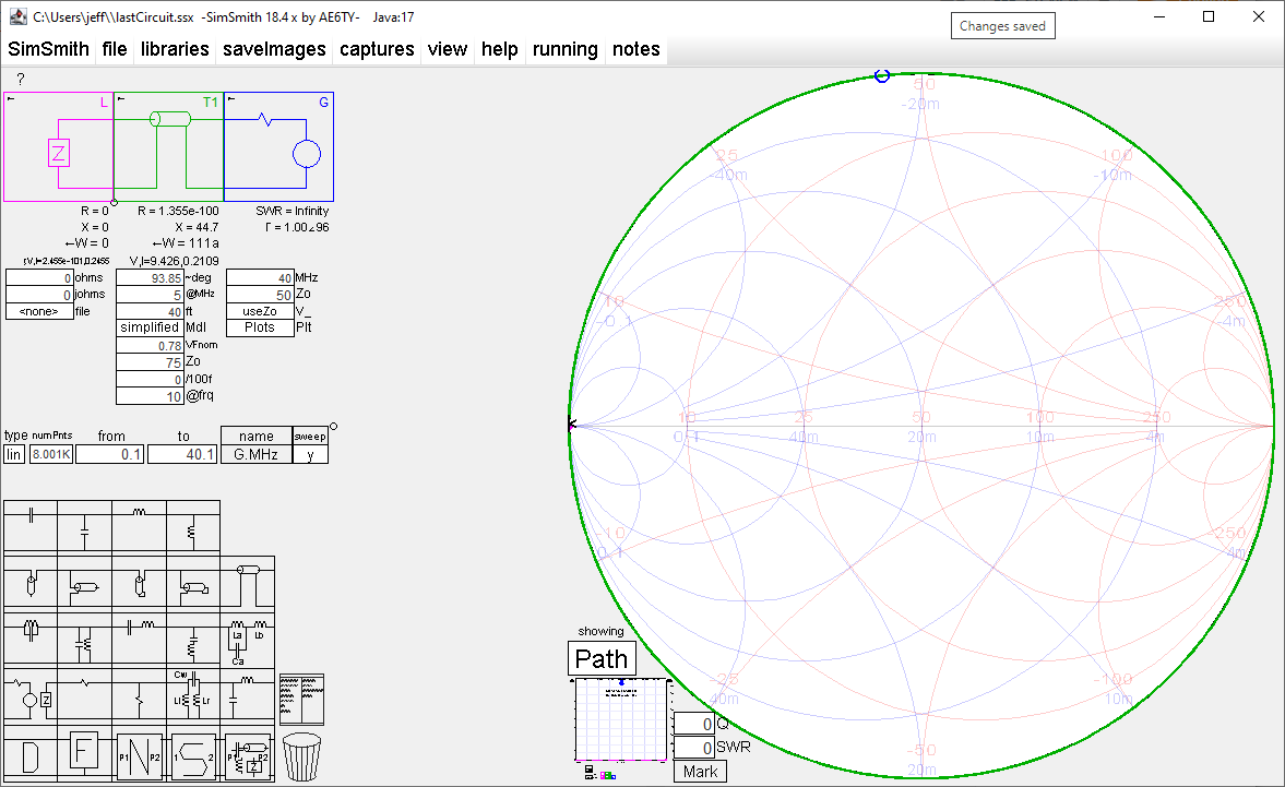
The example, shown below, shows circles of constant SWR for a transmission line whose Zo is 75 ohms and which, in one case, is terminated with 50 ohms, and in the other case terminated with 300 ohms.  You can see that the geometric means of impedances opposite each other on either unit circle calculate to be 75 ohms, the Zo of the transmission line, independent of which SWR circle is used.

Circles of Constant SWR for Lossy Lines:

If the line is lossy the plotted S11 values will no longer trace a perfect circle on the Smith Chart as frequency is varied.  Instead, they will form a spiral which spirals, as frequency increases, inwards towards the Zo of the lossy transmission line.

Thus, we no longer have perfect circles of constant SWR (we have a spiral, instead), and choosing two points opposite on the spiral (e.g. both on the real-only axis) will give us a calculated value close to the transmission line's actual Zo, but it will not be perfect.

The less the line loss, however, the more accurate the calculation will be.

Below is a plot showing a simulated example of Belden 8241 75 ohm coax terminated with 50 ohms.  Included is also the constant SWR circle (in yellow) for the same load, but assuming ideal, lossless, coax.

If the load is changed from 50 ohms to 300 ohms, the lossy coax's spiral is larger and thus more obvious.

But the calculation is very close to 75 ohms.  Not too bad!

Mathematics:

I won't go into the mathematical under-pinings too deeply.  Just recognize that the fundamental equation for analyzing this behavior is the equation for Zin for a terminated transmission line (whether the line be lossy or it be lossless).

If the line is lossless, α equals 0 and Γ (of the load) is only modified by a phase shift (its magnitude remains constant -- thus the "circle" of constant SWR).

For more on the math assuming lossless coax, see here.

If the line is lossy, well, then things get more complicated.  We have some of the same potential issues that we had with the 1/8th-Lambda technique (e.g. Zo being complex, not real-only).  So any calculation of Zo using this method should be considered an estimation (albeit perhaps a very good estimation), but there will be some amount of uncertainty, too.

If you have any question about your calculation, I would recommend recording several of the spiral loops and calculate Zo using multiple pairs of opposite-points to, hopefully, provide a more accurate Zo result.

But, despite its potential drawbacks, I have found that I can quickly make the measurement on a VNA and get a reasonable result for Zo.

Resources:

More on the underlying "lossless line" math can be found, here:  Munk, Ben A., Metamaterials: Critique and Alternatives, Wiley Online Library, Appendix C, How to Measure the Characteristic Impedance and Attenuation of a Cable

Standard Caveat:

As always, I might have made a mistake in my equations, assumptions, drawings, or interpretations.  If you see anything you believe to be in error or if anything is confusing, please feel free to contact me or comment below.

And so I should add -- this information is distributed in the hope that it will be useful, but WITHOUT ANY WARRANTY; without even the implied warranty of MERCHANTABILITY or FITNESS FOR A PARTICULAR PURPOSE. here

Transmission Lines: Measuring Zo, the Characteristic Impedance, Method 2: 1/8th Lambda

In my previous post (here) I described the method of determining a transmission line's Characteristic Impedance Zo from measurements of its input impedance when terminated with a short and when terminated with an open.

In this new post I will describe a second method that is sometimes used determine a transmission line's Zo  (such as in some versions of the NanoVNA's firmware).  I will call this second method the "1/8th-Lambda Method" (where "Lambda" is the wavelength of the signal on the transmission line).  I first learned of this method here.

The 1/8th-Lambda method uses S11 measurements of a transmission line, and these can be made with the line terminated either with an OPEN or with a SHORT.

Assuming the transmission line is terminated with an OPEN, the principle behind this technique is that the magnitude of the reactive-component 'Xin' of Zin, the terminated transmission line's input impedance (as calculated from S11), will equal Zo at a point 1/8th of a wavelength from the point at S11's phase passes through 180 degrees (or 0 degrees, if the transmission line is terminated with a SHORT).   

To find this 1/8th-Lambda point, assuming the line is terminated with an OPEN and the S11 frequency sweep is starting near 0 Hz:

1.  Find the frequency at which the phase of S11 is -180 degrees (on the left-hand side of the Smith Chart and on the x-axis).  This is the quarter-wavelength frequency of an OPEN-terminated transmission line.

2.  Divide this frequency by 2.  This new frequency is the eighth-wavelength frequency of the transmission line.  Note S11 at this point.

3.  Convert this S11 value to Zin (where Zin = Rin + jXin).  The value of Xin will be the negative of Zo, and therefore Zo = -Xin.

This same method can be used, with a few small changes, if the transmission line is terminated with a SHORT: 

1.  Find the frequency at which the phase of S11 is 0 degrees on the right-hand side of the Smith Chart.  This is the quarter-wavelength frequency for this length of transmission line (assuming the S11 scan starts near 0 Hz).

2.  Divide this frequency by 2.  This new frequency is the frequency for which the transmission line is an eighth of a wavelength long.  Note S11 at this point.

3.  Convert this S11 value to Zin (Zin = Rin + jXin).  The value of Xin will be the negative of Zo, and therefore Zo = -Xin.

DISCLAIMER:  This technique works best when the transmission line is essentially lossless.  Calculations made using measurements of lossy lines will have some amount of error.  I'll discuss this issue later in this post.

The 1/8-Lambda Method and Lossless Transmission Lines:

Let's look at the principle behind this technique assuming a lossless transmission line...

Example:  Lossless Transmission Line Terminated with an OPEN:

I've used SimSmith to model 40 feet of ideal (lossless) 75-ohm coax terminated with an OPEN.  The simulation parameters are in the image, below.

With this simulation I created an S11 file (frequency spanning from 1 KHz to 6.001 MHz.).  The S11 plot is shown below.  

Note that S11, the Reflection-Coefficient, curve passes through -180 degrees at about 4.057 MHz.  At this frequency the transmission-line is a quarter-wavelength long.

To find the eighth-wavelength point, we divide 4.057 MHz by 2, which results in a frequency of 2.0285 MHz.

Convert the measured S11 data for this frequency to Zin:  assuming the VNA is calibrated for 50 ohms, Zin = 50*(1+S11)/(1-S11).

At this point on the Smith Chart, above, (actually, close to it -- the S11 capture skips 2.0285 MHz), Zin = -4e-8 - j75.04 ohms

From the derivation above for an OPEN termination, Zin = -jZo, therefore Zo = jZin.

Substituting in the value of Zin and solving...

Zo = j*(-4e-8-j75.04) = 75.04 - j(-4e-8).  

The imaginary term is negligible.  Therefore:

Zo = 75.04 ohms.  

Example:  Lossless Transmission Line Terminated with a SHORT:

We can do a similar calculation if the transmission line is terminated with a SHORT.  Below is the Smith Chart showing the Reflection Coefficient path.

The 1/8th Lambda frequency is again 2.0285 MHz, and again we will use 2.028 MHz on the above Smith Chart.

Zin (calculated from the Reflection Coefficient) is -4e-8 + j74.96 ohms.

From the derivation above for a SHORT termination, Zin = jZo, therefore Zo = -jZin.

Substituting in the value of Zin and solving...

Zo = -j*(-4e-8 + j74.96) = 74.96 + j(4e-8).  

The imaginary term is again negligible, and thus:

Zo = 74.96 ohms.  

Conclusion:  For a lossless transmission line (or one whose loss is insignificant) the 1/8-Lambda method works quite well at finding Zo of the transmission line.  

The 1/8-Lambda Method and Lossy Transmission Lines:

How well does this technique perform if the line is lossy?

For a lossless transmission line, Zo is a real value and equal to the SQRT(L/C).  But for a lossy transmission line Zo is a complex value whose real and imaginary parts are both frequency dependent, as shown in the following two slides:

We can see the frequency-dependency of Zo's real and imaginary components in the following plot of Zo for Belden 8241 75 ohm coax.  The plotted Zo is calculated using Zo = SQRT(Zsc*Zoc), per the derivation in my previous blog post, using S11 files generated with SimSmith.

Below is the plot of S11 for 40 feet of Belden 8241 coax terminated with an OPEN.  Note that as frequency increases the Reflection Coefficient is spiraling in from the Smith Chart's unit-circle boundary.

In the plot below I have applied the 1/8-Lambda technique to two different S11 simulated-measurements.  In one measurement the 40 feet of Belden 8241 coax was terminated with an OPEN, and in the other it was terminated with a SHORT.

Using the same procedure that I used for the lossless line, the 1/8th-Lambda points are at 1.999 MHz (although there is some question as to this frequency -- more on this in a bit...).

Converting the S11 values at 1.999MHz to Zin, let's use the equations derived earlier (for a lossless line) to find Zo:

From the Smith Chart above, Zin at the 1/8th-Lambda points for the SHORT and the OPEN are:.

• For the OPEN termination, Zin  @ (1.999 MHz) = 1.721 - j75.98 ohms
• For the SHORT termination, Zin @ (1.999 MHz) = 7.595 + j75.56 ohms.

Using the above equations to transform Zin to Zo , the results are:

Zo (OPEN @ 1/8 Lambda) = 75.98 + j1.721 ohms

Zo (SHORT @ 1/8 Lambda) = 75.56 - j7.595 ohms

I would expect Zo calculated with this method to be approximately equal to the values found using the equation Zo = SQRT(Zsc*Zoc), which, per the plot below (at the 1/8th-Lambda frequency) are:  

Zo (@ 1.998 MHz) = 76.41 - j2.92 ohms

And the 'real' part of Zo is quite close (within about an ohm).  But the imaginary parts are significantly different -- the OPEN's Xo is positive, rather than negative, and the SHORT's Xo is more than twice the value calculated using Zo = SQRT(Zsc*Zoc).

So, although the results are certainly acceptable, I wonder what could be causing the discrepancies.  There are a number of assumptions implied with this method.  Are these assumptions valid?

1/8th-Lambda Lossy Transmission Line Questions and Concerns:

1.  The 1/8th-Lambda method assumes that the quarter-wavelength frequency is when the angle of S11 is -180 degrees (for an OPEN termination).  But for a lossy line, the quarter-wavelength point is not where S11's phase is -180 degrees.  Zo is a complex number for lossy lines, and thus Zin at 1/4 wavelength would also have some amount of reactance, meaning that S11, at 1/4 Lambda, will have an angle other than 180 or 0 degrees.  How much of a difference would this make?  I don't know.

2.  The 1/8th-Lambda method assumes that the frequency for the 1/8th wavelength is half the frequency of the quarter-wavelength.  But the velocity factor of lossy transmission lines is not a constant, but varies with frequency (see here and here).  

Therefore, a quarter-wavelength length of transmission line at one frequency will not be an eighth-wavelength at half that frequency.  How much difference does this make?  I don't know.

3.  Note that the imaginary component Xo (the reactance of the calculated Zo) is negative if the SHORT termination is used and positive if the OPEN termination is used.  This sign convention will always be the case, irrespective of Zo, as long as the line is lossy, because Rin is always positive, but it is multiplied by +j to calculate Zo for an OPEN termination and by -j to calculate Zo for a SHORT termination (see the Zin to Zo conversion equations for 1/8th-Lambda earlier in this post).

Thus, the sign of Xo (the reactance of Zo) depends upon the load being an open or a short, which makes this value questionable.

4.  If we increase frequency to a point where loss is small, do the results from the 1/8th-Lambda technique improve?

Below is an S11 plot of 40 feet of Belden 8241 75-ohm coax out to 100 MHz.

Note that the frequency where S11 crosses 0 degrees is about 88.901 MHz, and the frequency where S11 crosses 180 degrees is about 92.951 degrees.  The frequency half-way between these two frequencies is the 1/8th-lambda frequency, which, in this case, is 90.926 Mhz.

At this point S11 represents an input impedance, Zin, of 21.51-j72.29 ohms.

Given that the line is terminated with an OPEN, we use the following formula to convert Zin to Zo at the 1/8th-Lambda frequency:

Zo = -Xin + jRin = 72.29 + j21.51 ohms.

However, using the equation Zo = SQRT(Zsc*Zoc) at this frequency, Zo, per the plots below, calculates to be:

Zo = 75.3 - j0.29 ohms

So there seems to an error at high frequencies, too.

Lossy-Line Equations:

In addition to the uncertainty in the quarter-wave frequency and in the Velocity Factor, part of the problem is undoubtedly due to the equations derived for a lossless transmission line are a simplification of the equations for a lossy line.

Let's derive those equations...

Given the last equation, above, if α is known, then the equation for Zo can be modified.  But α for the lossy line would first need to be found.  Plus, there are still the unresolved issues of Zo being complex (and its angle at 1/4 Lambda, hence uncertainty in the quarter-wave frequency) as well as frequency-dependent Velocity Factor.

In other words, the one-eighth-Lambda technique might get you close to the actual Zo, but there will be some amount of error in the calculated value.

Conclusions:

1.  If the transmission line is lossy, expect some amount of error in your Zo calculation.  But you will probably be reasonably close to the transmission line's actual Zo.

Other Notes:

Owen Duffy has an interesting post on an alternate method for finding the 1/8th-Lambda frequency and its associated Zo.  See here.  

Essentially, he measures the impedances of both a shorted line and an open line, and then, at the frequency where the |X| values of the two measurements intersect, he identifies this frequency as the 1/8th-Lambda point and defines Zo to be equal to |X| at this frequency.

Resources:

Transmission Line stuff: https://122.physics.ucdavis.edu/sites/default/files/files/Electronics/TransmissionLinesPart_II.pdf

On frequency-dependent Velocity Factor: https://scholar.valpo.edu/cgi/viewcontent.cgi?filename=28&article=1000&context=engineering_oer&type=additional

and here:  https://owenduffy.net/transmissionline/concept/mvf/index.htm

Standard Caveat:

As always, I might have made a mistake in my equations, assumptions, drawings, or interpretations.  If you see anything you believe to be in error or if anything is confusing, please feel free to contact me or comment below.

And so I should add -- this information is distributed in the hope that it will be useful, but WITHOUT ANY WARRANTY; without even the implied warranty of MERCHANTABILITY or FITNESS FOR A PARTICULAR PURPOSE.

Transmission Lines: Measuring Zo, the Characteristic Impedance, Method 1: Zo=SQRT(Zsc*Zoc)

Recently there was an interesting thread on measuring the characteristic impedance of a transmission line (Zo), on the nanovna-users groups.io site

There are several ways Zo can be calculated using S11 measurements.  Owen Duffy discusses one method:  https://owenduffy.net/blog/?p=28623. This method uses two S11 captures to calculate Zo -- one capturing the transmission line's input impedance with the line terminated with a SHORT (i.e. Zin = Zsc), and the other capture with the line terminated with an OPEN (i.e. Zin = Zoc).  From these two measurements Zo can be calculated using the following formula:

Zo = SQRT(Zsc*Zoc)

Duffy's derivation uses tanh() and coth() functions.  I've always preferred using complex-exponential functions, rather than hyperbolic trigonometry, for transmission line calculations.  Either method will give the same results; it is just that I find using complex-exponentials more intuitive.  But each to their own taste!

So in this blog post I will derive Zo = SQRT(Zsc*Zoc) using the complex-exponential form of the equation for Zin, the input impedance of a terminated transmission line.  Please refer to the following images.

Note that the exponential terms in the equations for Zsc and Zoc cancel if the line-length for all measurements are identical.  Thus, if the transmission line lengths (including the short and open) are identical, this equation is independent of any non-ideal characteristic of the transmission line (e.g. loss).

And because of this requirement that the length of the transmission line be the same for both sets of S11 measurements.  I would not recommend just leaving the coax unterminated for the open measurement.  Ideally, you should use OPEN and SHORT calibration standards that have the same length (i.e. the same Offset Delay) from the connectors' Reference Plane to the actual short or open implemented within the standard.

Example, Finding Zo of Belden 75-ohm Coax:

In this example I'll use SimSmith to simulate two versions of 75 ohm coax -- one version of coax is perfect, without loss, and  the other version is Belden 9659 (which does have some loss) to demonstrate the calculation of Zo and to show the effect of loss on Zo.

Both lengths of simulated-coax are 40 feet long, and I will use SimSmith to create S11 files of the lines terminated with a short and with an open.

First, below is an S11 plot of the perfect 75 ohm coax terminated with a SHORT.  (The OPEN termination looks the same, except that it starts at "3 o'clock" on the Smith Chart).  Note how the path (in green) follows the boundary of the Smith Chart's unit circle.  In this case, SWR is always infinite.

Next is an S11 plot of the Belden 9659 75-ohm coax, terminated with a short.  Note that the path no longer follows the boundary of the Smith Chart's unit circle.  Instead, it spirals in (i.e. SWR improving as it spirals in).  This spiraling is due to coax-cable loss.

And here is the S11 plot of the same Belden 9659 75-ohm coax terminated with an OPEN.  Again, note the spiraling-in due to loss.

The following two plots show the calculation of Zo, from S11 data, using the SQRT(Zsc*Zoc) method.  Zo for both the perfect (lossless) transmission line and for the Belden 9659 75-ohm transmission line are shown.

The first plot is to 40 MHz.

And the second plot (to better show the Belden cable's Zo at low frequency) is to 4 MHz.

Note that Zo of the perfect coax is 75 + j0 ohms irrespective of frequency.  However, the Belden coax always has a reactive (imaginary) component (whose value decreases as frequency increases), and at lower frequencies its Zo deviates appreciably from the ideal 75 ohms.

What causes this deviation from 75 ohms, especially at low frequencies?

A transmission line's Zo is due to four physical characteristics of the transmission line:  resistance, conductance, inductance, and capacitance, per the equation in the image, below.

If the numerator and denominator under the top equation's square root are expanded, they will form a 'real' term and an 'imaginary' term -- that is, a complex number.  A square-root of a complex number is a complex number, and thus a transmission line's characteristic impedance is always a complex value.

At lower frequencies the greater will be the effect of the loss factors R and G on the real and imaginary components of Zo.  This effect can be seen in  the plots, above.

However, if the frequency is high enough, or if R and G are negligible, we can approximate Zo as a 'real' value, without any imaginary component.

Real-World Issues:

There was recently an interesting discussion about this method on the nanovan-users group, here.

François, F1AMM, posted the following image showing his calculation of the real part of Zo, where Zo was calculated using his measurements of Zsc and Zoc.  It does not look anything like my SimSmith-simulated curves, above.

Why the difference?

I took my SimSmith-simulated Zsc and Zoc files for RG-142B and, using MATLAB, applied a frequency-dependent phase shift to S11 of one of the files (simulating an additional delay on that line).  The result is plotted below:

This was revealing, and I suspect that François' measurements were the result of his SHORT and OPEN standards being different lengths.

I was curious if my homebrew SMA standards would perform better, and so I measured Zsc and Zoc of a 10 foot length of RG-142B using both my NanoVNA and my HP 8753C.  The Zo-calculation results are shown below.

The errors aren't as dramatic as those of François, but they are greater than I had expected.  What could be their cause?

To explore further, I wrote a MATLAB routine that simulated a transmission line and a "virtual" VNA, to allow me to simulate a 75-ohm transmission line with the following test options:

1. Calibrate the "virtual" VNA with Actual or Ideal SOL standards
2. Set the SOL Characteristics (within a "virtual VNA") to be their actual characteristics or their ideal characteristics.
3. Terminate the simulated coax with a Short or an Open whose characteristics are either actual or ideal.
4. Play around with various "actual" SOL parameters (e.g. capacitance of the Open, inductance of the Short, resistance of the Load, "Offset Delays" of each (see here for explanation).

The MATLAB simulation can be downloaded from:

https://github.com/k6jca/Simulation_of_Zo_sqrt-ZscZoc-_calculation

The following plots are the results of some of these simulations.

First, verifying the simulation by calculating Zo assuming the SOL standards and the line-terminations are perfect.  Not surprisingly, the plot looks as it should.

Next, I changed the LOAD standard from being a perfect 50 ohms to 51 ohms (i.e. it has 40 dB Return Loss), but keeping the VNA's characterization of the load at a perfect 50 ohms.  

The results surprised me.  After all, how many of us run our VNAs this way -- assume that the LOAD, even though it might not be exactly 50 ohms, is close enough?

Next, I simulated the "virtual" VNA being calibrated with perfect standards, but the Zsc and Zoc measurements made with imperfect terminations (the OPEN had 50 femtoFarads of capacitance plus an offset-delay of 17.5 picoseconds, while the SHORT, although have no inductance, had 17.8 picoseconds of offset-delay).

I wondered if we could remove the plotted-error by using the imperfect SHORT's and OPEN's actual characteristics in the "virtual" VNA for calibration.  Note that the LOAD was assumed to a perfect 50 ohms.

The result still had errors. 

Finally, I ran a simulation in which the SOL standards were assumed by the "virtual" VNA to be perfect (i.e. their Characterizations), but the imperfect standards were used for calibration and for the Zsc and Zoc measurements, to simulate how I suspect many users (such as me) use their NanoVNAs).

Not surprisingly, there are still errors.

Conclusion:

The "SQRT(Zsc*Zoc)" method of calculating Zo will theoretically calculate accurate real and imaginary components of a transmission line's Zo. 

However, from my plots above, in reality there always will be some amount of error in the Zo calculation, because it is impossible for the SHORT and OPEN standards to be perfect, and these imperfections cannot be calibrated away for the purposes of this method of Zo calculation.

Some Useful Links:

Determination of transmission line characteristic impedance from impedance measurements.  Owen Duffy blog post discussing this method of finding Zo.

Waves on Transmission Lines. (Useful on-line course notes from Sacramento State).

Section 2.3, The Terminated Lossless Line.  From on-line libretext.  (Note error in the derivation of equation 2.3.18 -- cos() is shown in the imaginary term.  This should be sin()).

Section 2.5, The Lossy Terminated Line.  From on-line libretext.  (Note error in the derivation of equation 2.5.5 -- cosh() is shown in the imaginary term.  This should be sinh()).

Standard Caveat:

As always, I might have made a mistake in my equations, assumptions, drawings, or interpretations.  If you see anything you believe to be in error or if anything is confusing, please feel free to contact me or comment below.

And so I should add -- this information is distributed in the hope that it will be useful, but WITHOUT ANY WARRANTY; without even the implied warranty of MERCHANTABILITY or FITNESS FOR A PARTICULAR PURPOSE.

Transmission Lines: Input Impedance of a Terminated Line

A common equation for calculating Zin of a terminated transmission line uses complex exponentials.  But now and again I come across an equivalent equation that instead uses the hyperbolic tangent function, tanh().

I have never used hyperbolic trig functions as an engineer -- in fact, the only time I've come across them is with respect to transmission lines, and personally, I find the complex-exponential form of these equations much more intuitive, given how common complex exponentials are used in electrical engineering.

This blog post shows how the tanh() form of the equation for Zin, the input impedance of a terminated lossy transmission line, can be derived from the complex-exponential equation.

Also, I will show how, for a lossless transmission line, the tanh() equation reduces to one using tangent (tan()) functions.

I'll start out this post with the lossy-line's complex-exponential equation for Zin, which is:

Zin = Zo*(1 + Γ*e^(-2*γ*l)) / (1 - Γ*e^(-2*γ*l)),

where Γ = (Zload - Zo) / (Zload + Zo),  γ = α + jβ, and l = length.  Note that α represents loss and jβ represents phase-shift as a signal travels along a transmission line.

And later in this post I'll do the same for the lossless line, whose complex-exponential equation is:

Zin = Zo*(1 + Γ*e^(-j2*β*l)) / (1 - Γ*e^(-j2*β*l)),

which is the same equation is the first one, above, but with α (which represents loss) set to 0.

The rest will be explained in the following slides...

That's it!

Standard Caveat:

As always, I might have made a mistake in my equations, assumptions, drawings, or interpretations.  If you see anything you believe to be in error or if anything is confusing, please feel free to contact me or comment below.

And so I should add -- this information is distributed in the hope that it will be useful, but WITHOUT ANY WARRANTY; without even the implied warranty of MERCHANTABILITY or FITNESS FOR A PARTICULAR PURPOSE.