Transmission Lines: Measuring Zo, the Characteristic Impedance, Method 1: Zo=SQRT(Zsc*Zoc)

Recently there was an interesting thread on measuring the characteristic impedance of a transmission line (Zo), on the nanovna-users groups.io site

There are several ways Zo can be calculated using S11 measurements.  Owen Duffy discusses one method:  https://owenduffy.net/blog/?p=28623. This method uses two S11 captures to calculate Zo -- one capturing the transmission line's input impedance with the line terminated with a SHORT (i.e. Zin = Zsc), and the other capture with the line terminated with an OPEN (i.e. Zin = Zoc).  From these two measurements Zo can be calculated using the following formula:

Zo = SQRT(Zsc*Zoc)

Duffy's derivation uses tanh() and coth() functions.  I've always preferred using complex-exponential functions, rather than hyperbolic trigonometry, for transmission line calculations.  Either method will give the same results; it is just that I find using complex-exponentials more intuitive.  But each to their own taste!

So in this blog post I will derive Zo = SQRT(Zsc*Zoc) using the complex-exponential form of the equation for Zin, the input impedance of a terminated transmission line.  Please refer to the following images.

Note that the exponential terms in the equations for Zsc and Zoc cancel if the line-length for all measurements are identical.  Thus, if the transmission line lengths (including the short and open) are identical, this equation is independent of any non-ideal characteristic of the transmission line (e.g. loss).

And because of this requirement that the length of the transmission line be the same for both sets of S11 measurements.  I would not recommend just leaving the coax unterminated for the open measurement.  Ideally, you should use OPEN and SHORT calibration standards that have the same length (i.e. the same Offset Delay) from the connectors' Reference Plane to the actual short or open implemented within the standard.

Example, Finding Zo of Belden 75-ohm Coax:

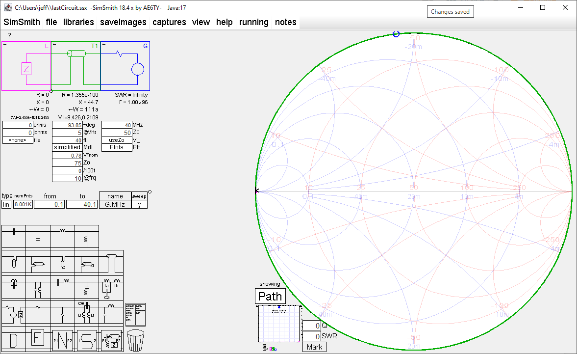
In this example I'll use SimSmith to simulate two versions of 75 ohm coax -- one version of coax is perfect, without loss, and  the other version is Belden 9659 (which does have some loss) to demonstrate the calculation of Zo and to show the effect of loss on Zo.

Both lengths of simulated-coax are 40 feet long, and I will use SimSmith to create S11 files of the lines terminated with a short and with an open.

First, below is an S11 plot of the perfect 75 ohm coax terminated with a SHORT.  (The OPEN termination looks the same, except that it starts at "3 o'clock" on the Smith Chart).  Note how the path (in green) follows the boundary of the Smith Chart's unit circle.  In this case, SWR is always infinite.

Next is an S11 plot of the Belden 9659 75-ohm coax, terminated with a short.  Note that the path no longer follows the boundary of the Smith Chart's unit circle.  Instead, it spirals in (i.e. SWR improving as it spirals in).  This spiraling is due to coax-cable loss.

And here is the S11 plot of the same Belden 9659 75-ohm coax terminated with an OPEN.  Again, note the spiraling-in due to loss.

The following two plots show the calculation of Zo, from S11 data, using the SQRT(Zsc*Zoc) method.  Zo for both the perfect (lossless) transmission line and for the Belden 9659 75-ohm transmission line are shown.

The first plot is to 40 MHz.

And the second plot (to better show the Belden cable's Zo at low frequency) is to 4 MHz.

Note that Zo of the perfect coax is 75 + j0 ohms irrespective of frequency.  However, the Belden coax always has a reactive (imaginary) component (whose value decreases as frequency increases), and at lower frequencies its Zo deviates appreciably from the ideal 75 ohms.

What causes this deviation from 75 ohms, especially at low frequencies?

A transmission line's Zo is due to four physical characteristics of the transmission line:  resistance, conductance, inductance, and capacitance, per the equation in the image, below.

If the numerator and denominator under the top equation's square root are expanded, they will form a 'real' term and an 'imaginary' term -- that is, a complex number.  A square-root of a complex number is a complex number, and thus a transmission line's characteristic impedance is always a complex value.

At lower frequencies the greater will be the effect of the loss factors R and G on the real and imaginary components of Zo.  This effect can be seen in  the plots, above.

However, if the frequency is high enough, or if R and G are negligible, we can approximate Zo as a 'real' value, without any imaginary component.

Real-World Issues:

There was recently an interesting discussion about this method on the nanovan-users group, here.

François, F1AMM, posted the following image showing his calculation of the real part of Zo, where Zo was calculated using his measurements of Zsc and Zoc.  It does not look anything like my SimSmith-simulated curves, above.

Why the difference?

I took my SimSmith-simulated Zsc and Zoc files for RG-142B and, using MATLAB, applied a frequency-dependent phase shift to S11 of one of the files (simulating an additional delay on that line).  The result is plotted below:

This was revealing, and I suspect that François' measurements were the result of his SHORT and OPEN standards being different lengths.

I was curious if my homebrew SMA standards would perform better, and so I measured Zsc and Zoc of a 10 foot length of RG-142B using both my NanoVNA and my HP 8753C.  The Zo-calculation results are shown below.

The errors aren't as dramatic as those of François, but they are greater than I had expected.  What could be their cause?

To explore further, I wrote a MATLAB routine that simulated a transmission line and a "virtual" VNA, to allow me to simulate a 75-ohm transmission line with the following test options:

1. Calibrate the "virtual" VNA with Actual or Ideal SOL standards
2. Set the SOL Characteristics (within a "virtual VNA") to be their actual characteristics or their ideal characteristics.
3. Terminate the simulated coax with a Short or an Open whose characteristics are either actual or ideal.
4. Play around with various "actual" SOL parameters (e.g. capacitance of the Open, inductance of the Short, resistance of the Load, "Offset Delays" of each (see here for explanation).

The MATLAB simulation can be downloaded from:

https://github.com/k6jca/Simulation_of_Zo_sqrt-ZscZoc-_calculation

The following plots are the results of some of these simulations.

First, verifying the simulation by calculating Zo assuming the SOL standards and the line-terminations are perfect.  Not surprisingly, the plot looks as it should.

Next, I changed the LOAD standard from being a perfect 50 ohms to 51 ohms (i.e. it has 40 dB Return Loss), but keeping the VNA's characterization of the load at a perfect 50 ohms.  

The results surprised me.  After all, how many of us run our VNAs this way -- assume that the LOAD, even though it might not be exactly 50 ohms, is close enough?

Next, I simulated the "virtual" VNA being calibrated with perfect standards, but the Zsc and Zoc measurements made with imperfect terminations (the OPEN had 50 femtoFarads of capacitance plus an offset-delay of 17.5 picoseconds, while the SHORT, although have no inductance, had 17.8 picoseconds of offset-delay).

I wondered if we could remove the plotted-error by using the imperfect SHORT's and OPEN's actual characteristics in the "virtual" VNA for calibration.  Note that the LOAD was assumed to a perfect 50 ohms.

The result still had errors. 

Finally, I ran a simulation in which the SOL standards were assumed by the "virtual" VNA to be perfect (i.e. their Characterizations), but the imperfect standards were used for calibration and for the Zsc and Zoc measurements, to simulate how I suspect many users (such as me) use their NanoVNAs).

Not surprisingly, there are still errors.

Conclusion:

The "SQRT(Zsc*Zoc)" method of calculating Zo will theoretically calculate accurate real and imaginary components of a transmission line's Zo. 

However, from my plots above, in reality there always will be some amount of error in the Zo calculation, because it is impossible for the SHORT and OPEN standards to be perfect, and these imperfections cannot be calibrated away for the purposes of this method of Zo calculation.

Some Useful Links:

Determination of transmission line characteristic impedance from impedance measurements.  Owen Duffy blog post discussing this method of finding Zo.

Waves on Transmission Lines. (Useful on-line course notes from Sacramento State).

Section 2.3, The Terminated Lossless Line.  From on-line libretext.  (Note error in the derivation of equation 2.3.18 -- cos() is shown in the imaginary term.  This should be sin()).

Section 2.5, The Lossy Terminated Line.  From on-line libretext.  (Note error in the derivation of equation 2.5.5 -- cosh() is shown in the imaginary term.  This should be sinh()).

Standard Caveat:

As always, I might have made a mistake in my equations, assumptions, drawings, or interpretations.  If you see anything you believe to be in error or if anything is confusing, please feel free to contact me or comment below.

And so I should add -- this information is distributed in the hope that it will be useful, but WITHOUT ANY WARRANTY; without even the implied warranty of MERCHANTABILITY or FITNESS FOR A PARTICULAR PURPOSE.