The equations presented in this blog post can be used to design L-Networks that will transform any complex load impedance to be any other complex impedance.
The only assumptions are:
1. The L-Network is lossless (equations for lossy L-Networks are much more complex, see: Lossy L-Network Equations).
2. The 'real' component of the impedances cannot be negative.
These equations represent a continuation of the equations I had derived for transforming a complex load to a real (with no imaginary component) impedance (see either L-Network Equations or my article, "Correcting a Common L-Network Misconception," in the 2023 March-April issue of QEX magazine).
A Quick Review: The Eight L-Network Configurations:
Note that there are 8 possible L-Network configurations, divided into 4 Series-Parallel L-Networks and 4 Parallel-Series L-Networks:


Equations for Series-Parallel L-Network Solutions:

Depending upon the particular desired impedance transformation, there will be either two different Series-Parallel L-Network solutions for that impedance transformation, a single Series-Parallel solution, or no Series-Parallel solution. We can determine which of these results will be true by using the following criteria:

The equations for calculating a Series-Parallel L-Network's X and B values are listed, below. Note that there are two sets of X and B equations, meaning that there is the possibility of two different Series-Parallel L-Network solutions for a particular impedance transformation.

The signs of the calculated values of X and B determine the type of Series-Parallel L-Network represented by each X, B pair:


Equations for Parallel-Series L-Network Solutions:

Depending upon the particular desired impedance transformation, there will be either two different Parallel-Series L-Network solutions for that impedance transformation, a single Parallel-Series solution, or no Parallel-Series solution. We can determine which of these results will be true by using the following criteria:
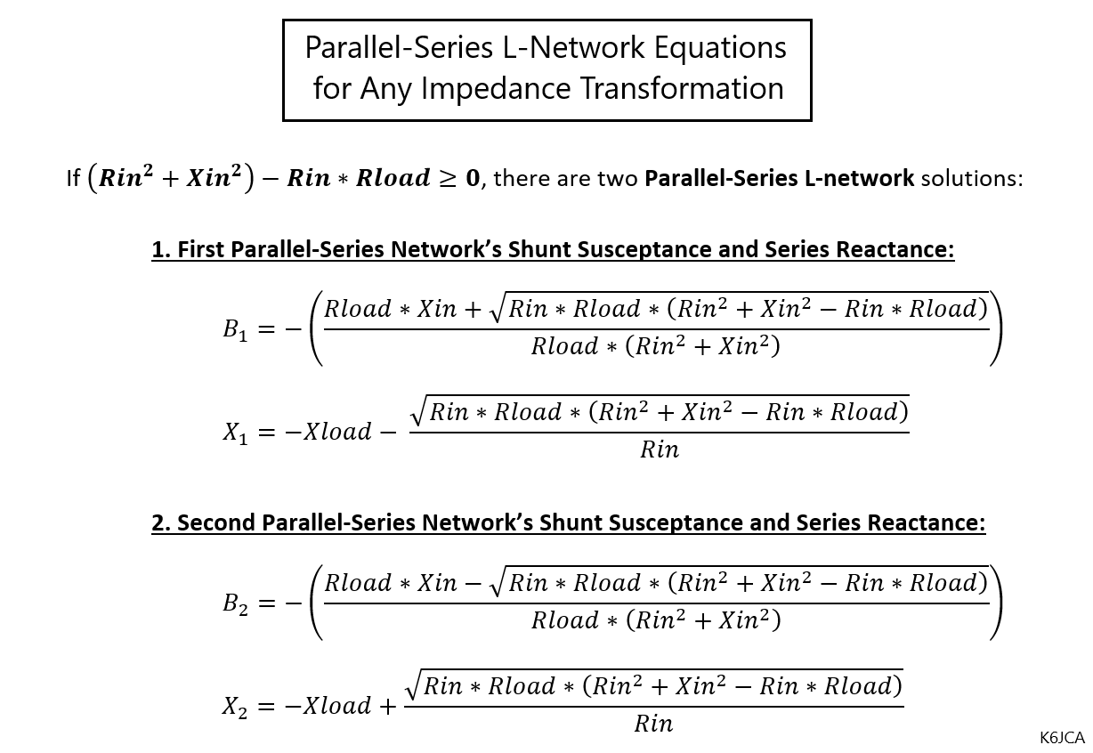
The equations for calculating a Parallel-Series L-Network's B and X values are listed, below. Note that there are two sets of B and X equations, meaning that there is the possibility of two different Parallel-Series L-Network solutions for a particular impedance transformation.

The signs of the calculated values of B and X determine the type of Parallel-Series L-Network represented by each B, X pair:


I had no success in my attempt to derive the above equations by hand. However, MATLAB and its Symbolic Math Toolbox can go where this mere human cannot. Dick Benson, W1QG, a good friend and MATLAB expert, showed me how MATLAB and its Symbolic Math Toolbox can derive these equations.
Below is a MATLAB script that will derive these equations.
% *****
% L_Network_Equation_Derivation_k6jca_V1
%
% Symbolic Math derivation of L network equations when
% Zin (looking into the L-Network) is defined to be a
% complex impedance rather than an impedance that is
% resistive only, with no reactance.
%
% Inspired by the MATLAB solution by Dick Benson, W1QG.
% See "RF Impedance Matching Application" at:
% https://www.mathworks.com/matlabcentral/profile/authors/6564033
%
% k6jca
% *****

clear; close; clc;

% Define the symbols in the equations.  Note:
% B is the susceptance of the L-Network shunt component.
% X is the reactance of the L-Network series component.
% Rld and Xld are the resistance and reactance of the load.
syms B X Rin Xin Rld Xld real

% *****
% Derive the Series-Parallel L-Network Equations
%
% Start by defining the equation for Zin given the
% Series-Parallel L-Network terminated with Zld = Rld+jXld:
fprintf('\nSeries-Parallel L-Network:\n')
Zin = 1i*X + 1/(1i*B + 1/(Rld + 1i*Xld))

% Next, solve the equation for B and X, given Zin = Rin+jXin
S_SP = solve(Zin==Rin+1i*Xin,[B,X],'ReturnConditions',true);

% Then, use 'simplify()' to simplify the resulting equations
series_par_B  = simplify(S_SP.B,'Steps',50);
series_par_X  = simplify(S_SP.X,'Steps',50);

% Finally, print the Series-Parallel X, B equation-pairs
fprintf('\nFirst Series-Parallel X, B pair:\n')
series_par_X1 = series_par_X(1,1)
series_par_B1 = series_par_B(1,1)
fprintf('\nSecond Series-Parallel X, B pair:\n')
series_par_X2 = series_par_X(2,1)
series_par_B2 = series_par_B(2,1)

% *****
% Derive the Parallel-Series L-Network Equations
%
% Start by defining the equation for Zin given the
% Parallel-Series L-Network terminated with Zld = Rld+jXld:
fprintf('\n\n\nParallel-Series L-Network:\n')
Zin = 1/(1i*B + 1/(Rld + 1i*Xld + 1i*X))

% Next, solve the equation for B and X, given Zin = Rin+jXin
S_PS = solve(Zin==Rin+1i*Xin,[B,X],'ReturnConditions',true);

% Then, use 'simplify()' to simplify the resulting equations
par_series_B  = simplify(S_PS.B,'Steps',50);
par_series_X  = simplify(S_PS.X,'Steps',50);

% Finally, print the Parallel-Series B, X equation-pairs
fprintf('\nFirst Parallel-Series B, X pair:\n')
par_series_B1 = par_series_B(1,1)
par_series_X1 = par_series_X(1,1)
fprintf('\nSecond Parallel-Series B, X pair:\n')
par_series_B2 = par_series_B(2,1)
par_series_X2 = par_series_X(2,1)

% END OF SCRIPT
Thanks!
A huge thanks to Dick Benson, W1QG, who took the equations I had derived for my article in the 2023 March-April issue of QEX and extended that concept to L-Network equations that can transform any complex impedance to any other complex impedance (not just to a real-only impedance).
Standard Caveat:
As always, I might have made a mistake in my equations, assumptions,
drawings, or interpretations. If you see anything you believe to be in
error or if anything is confusing, please feel free to contact me or comment
below.
And so I should add -- this information is distributed in
the hope that it will be useful, but WITHOUT ANY WARRANTY; without even the
implied warranty of MERCHANTABILITY or FITNESS FOR A PARTICULAR PURPOSE.


