Notes on Antenna Tuners: The Elecraft T1 (by Kai Siwiak, KE4PT)

In addition to his analysis of the Icom AH-4 Tuner, Kai Siwiak has also analyzed the Elecraft T1  Automatic Antenna Tuner.  With his permission, his analysis appears, below:

Elecraft T1 Automatic Tuner 

Kai Siwiak, KE4PT 

Tuner Description:

The Elecraft T1 tuner is an L-network tuner whose variable inductance is in series between the Radio-side and the Antenna-side ports of the tuner.  This inductance consists of 7 fixed inductors that allow the inductance to be varied from 0 to 7.5 uH in 0.05 uH steps.  The tuner's variable capacitance consists of 7 fixed capacitors that allow the capacitance to be varied from 0 to 1300 pF in 10 pF steps .  This variable capacitance can be switched to connect either between the tuner's input and ground, or between the tuner's output and ground.

These seven fixed inductors and seven fixed capacitors, along with the ability to connect the capacitance to either the input or the output of the tuner, are switched with latching relays, and results in a total of 2^7 x 2^7 x 2 = 32,768 different tuning combinations.  

Latching relays are used so the tuner draws no power from the battery except when tuning. 

A Stockton bridge circuit detects forward and reflected power, from which the SWR is calculated. A modulated SSB transmission can be used for tuning, with almost as good accuracy as a constant carrier. 

The microprocessor tries a coarse tuning algorithm to roughly determine the antenna impedance. This is followed by fine and very fine algorithms to seek the best possible match (unlike many auto-ATUs which stop searching once they have achieved an SWR below a certain level). The settings and band are stored, allowing the T1 to return to this setting instantly the next time that band is used. 

Unlike many other auto-ATUs, the T1 is switched off once it has found a match.  Thus, it does not constantly monitor the SWR in order to automatically re-tune if the SWR changes. The user must manually initiate a re-tune if required. 

The T1 can also be turned on using the external control interface, which can provide information about the band selected on the transceiver, allowing the T1 to automatically tune the antenna using the previously stored settings. Currently, this is only possible with the Yaesu FT-817 transceiver and optional adapter, but Elecraft has provided information about the serial data protocol used, to allow interfaces for other low-power transceivers to be designed. source: http://www.g4ilo.com/t1.html 

Tuner Analysis:

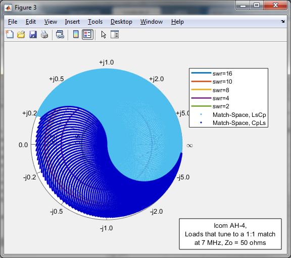
I terminated the “Radio side” of the tuner with a "perfect" 50 ohm resistor and used MathCAD to calculate the impedances on the “Antenna side” while stepping through the allowed component values (both L and C) for two cases:  1) the 0 – 1300 pF capacitor bank on the Antenna-side of the tuner, then 2), this same capacitor bank connected to the Radio-side of the tuner.  

I then plotted on a Smith chart the complex conjugate of the calculated impedances on the “Antenna side”.  This represents the impedances, when connected to the Antenna-side of the tuner, that the T1 can match to an SWR of 1:1.

Analysis covers the ham bands from 1.8 to 54 MHz.

Please note:

Assuming that the frequency derivative of the antenna impedance is not so large that the tuning algorithm can’t home in on it … 

• The 32,768 blue and magenta points on the Smith charts show which impedances at the tuner antenna port can be transformer to 50 ohms 
• 16,384 Blue points are for the bank of Caps on the antennas side 
• 16,384 Magenta points are for the bank of Caps on the transmitter side 

If there is a length of coax between the tuner and the radiator … 

• The coax losses will increase slightly 
• The points indicated on the Smith chart would need to be rotated counter-clockwise at a rate of one turn per electrical effective half wavelength of coax.

The range of input SWRs that the T-1 can match to an SWR of 1:1 on 160 and 80 meters is limited, as shown in the plots, below.  The T1's designer, Wayne Burdick, N6KR, says that a constructor whose interests lean towards LF could double the value of each inductor to improve the matching range on 160m, at the expense of 6m. 

Some Additional Notes (by Jeff, K6JCA)

1.  Actual component values (due to manufacturing tolerances, etc.) will manifest as unequal spacing between some of the impedances mapped onto the Smith Chart, compared to the simulated values.  (For an example, compare the two plots below from:  k6jca -- KAT500 notes).

2.  The L-network is assumed to be lossless.  In reality, there will be some loss, and this loss introduces errors into the "complex-conjugate" technique that both Kai and I (in other posts) use to calculate the impedances that the tuner will match.  You can find more on this topic in my Drake MN-4 post:  k6jca -- Drake MN-4.  Look for the subheading "Using MATLAB to Examine Loss Effects in Match-space Plots", towards the end of the post.

3.  On 6 meters the T1 might have a difficult timing finding an acceptable match, given the parts values listed in its Bill of Materials.  The plot below shows the best SWR that loads with an SWR of 10:1 (or better) can be tuned to at 54 MHz.  (The outer ring of the "donut" represents loads with a 10:1 SWR, while the inner ring represents loads with a 1.5:1 SWR.)

And below is the same plot for 30 MHz.  All loads with an SWR of 10:1 or better now tune to SWRs better than 2:1 (per the scale on the right-hand side).

And a plot for 3.5 MHz:

Plots made using the MATLAB code discussed here:  k6jca - 3D Smith Charts.

- Jeff, k6jca

Antenna Tuner Blog Posts:

A quick tutorial on Smith Chart basics:
http://k6jca.blogspot.com/2015/03/a-brief-tutorial-on-smith-charts.html

Plotting Smith Chart Data in 3-D:
http://k6jca.blogspot.com/2018/09/plotting-3-d-smith-charts-with-matlab.html

The L-network:
http://k6jca.blogspot.com/2015/03/notes-on-antenna-tuners-l-network-and.html

A correction to the usual L-network design constraints:
http://k6jca.blogspot.com/2015/04/revisiting-l-network-equations-and.html

Calculating L-Network values when the components are lossy:
http://k6jca.blogspot.com/2018/09/l-networks-new-equations-for-better.html

A look at highpass T-Networks:
http://k6jca.blogspot.com/2015/04/notes-on-antenna-tuners-t-network-part-1.html

More on the W8ZR EZ-Tuner:
http://k6jca.blogspot.com/2015/05/notes-on-antenna-tuners-more-on-w8zr-ez.html  (Note that this tuner is also discussed in the highpass T-Network post).

The Elecraft KAT-500:
http://k6jca.blogspot.com/2015/05/notes-on-antenna-tuners-elecraft-kat500.html

The Nye Viking MB-V-A tuner and the Rohde Coupler:
http://k6jca.blogspot.com/2015/05/notes-on-antenna-tuners-nye-viking-mb-v.html

The Drake MN-4 Tuner:
http://k6jca.blogspot.com/2018/08/notes-on-antenna-tuners-drake-mn-4.html

The Icom AH-4 Tuner (by Kai Siwiak, KE4PT):
http://k6jca.blogspot.com/2021/03/notes-on-antenna-tuners-icom-ah-4-by.html

The Elecraft T1 Tuner (by Kai Siwiak, KE4PT):
https://k6jca.blogspot.com/2021/03/notes-on-antenna-tuners-elecraft-t1-by.html

Measuring a Tuner's "Match-Space":
http://k6jca.blogspot.com/2018/08/notes-on-antenna-tuners-determining.html

Measuring Tuner Power Loss:
http://k6jca.blogspot.com/2018/08/additional-notes-on-measuring-antenna.html

Standard Caveat:

I might have made a mistake in my designs, equations, schematics, models, etc. If anything looks confusing or wrong to you, please feel free to comment below or send me an email.

Also, I will note:

This design and any associated information is distributed in the hope that it will be useful, but WITHOUT ANY WARRANTY; without even the implied warranty of MERCHANTABILITY or FITNESS FOR A PARTICULAR PURPOSE.

Notes on Antenna Tuners: The Icom AH-4 (by Kai Siwiak, KE4PT)

Kai Siwiak, KE4PT, forwarded to me his analysis of the Icom AH-4 Remote Tuner.  With his permission I have added it to this blog.

Icom AH-4 Tuner Analysis and Performance

Kai Siwiak, KE4PT

I analyzed the Icom AH-4 tuner using the circuit of Figure 1.  

Tuner Analysis:

I terminated the “Radio side” of the tuner with a "perfect" 50 ohm resistor and used MathCAD to calculate the impedances on the “Antenna side” while stepping through the allowed component values (both L and C) for two cases (0 – 2400 pF capacitor bank on the output, then on the input), and across ham bands from 1.8 to 54 MHz.

I then plotted on a Smith chart the complex conjugate of the calculated impedances on the “Antenna side”.  This maps the impedances that the AH-4 can match, given the range of component values in Figure 1. Figure 2 shows the range of impedances the AH-4 can match plotted on a Smith chart.  

Notice how the coverage on the Smith chart gets whittled away as the frequency decreases. It indicates that the component values do not have sufficient range to cover the whole chart at those frequencies!

Impedance coverage is not continuous, but depends on the step size of the components, and that granularity is revealed here by the inductor and capacitor steps in Figure 1.  

What this implies is that the tuner range of matching can be completely specified by: 

(1) the tuner topology, here in Figure 1, a reversible L network with additional switched capacitance on the antenna side; 

(2) the range of component values and the component step size; usually the minimum value of the inductor and minimum value of the capacitor in the capacitor bank. 

Also what is not revealed here is the tuning algorithm and tuning strategy. These are typically proprietary features. Given estimates of the inductor Q it would be possible to calculate the tuner losses across the Smith chart at various frequencies. The AH-4 inductors are air-wound, so will be lower loss than ferrite inductors.  

On tuning strategy, the AH-4 initially sets the connected compatible radio RF power to 10 W, and switches in a 10 dB attenuator between the radio and the tuner. Thus no more than 1 W is every supplied to the antenna during tuning, and the radio transmitter always “sees” more than 20 dB return loss (SWR < 1.2:1) during the tuning process, ensuring a valid tuning solution.  

I have similarly analyzed the Elecraft T1 miniature ATU, which also uses a reversible L network with 0 to 1300 pF by 10 pF and 0 to 7.5 uH by 0.055 uH (32,768 combinations). Its range of component values is smaller than that of the AH-4, so it cover less of the Smith chart. Its inductors are not air core, so losses will be higher than with the AH-4.  

Kindest regards, 

Kai Siwiak, KE4PT

Some Additional Notes (by Jeff, K6JCA)

To verify Kai's calculations, I analyzed the AH-4 using a MATLAB script I had written for analyzing tuners (e.g. the KAT-500).  If you compare my plotted results, below, with Kai's Figure 2, you will see that they match quite well.

And here's a plot at 54 MHz.  You can see the effect of component step-size:

Some notes regarding these plots:

1.  Step-size is assumed to be uniform.  But in reality this is not the case -- component values might have been selected for their ability to be sourced, rather than their "ideal" value, and these component values will also have tolerances.  (See the plots towards the end of the KAT500 analysis for the effect of "real" components upon a tuner's match-space:  k6jca -- KAT500 notes).

2.  I have ignored the 13 pF and the 100 pF capacitors that can be switched in and out of the circuit at the Antenna connector side of the tuner.  I suspect these are used to compensate for parasitic impedances when the tuner is in the CpLs mode, or possibly they bring the tuner's SWR close to 1:1 when the tuner is in "bypass" mode).

3.  The network is assumed to be lossless.  In reality, there will be some loss, and this loss introduces errors into the "complex-conjugate" technique that both Kai and I use to calculate the impedances that the tuner will match.  You can find more on this topic in my Drake MN-4 post:  k6jca -- Drake MN-4.  Look for the subheading "Using MATLAB to Examine Loss Effects in Match-space Plots", towards the end of the post.

- Jeff, k6jca

Antenna Tuner Blog Posts:

A quick tutorial on Smith Chart basics:
http://k6jca.blogspot.com/2015/03/a-brief-tutorial-on-smith-charts.html

Plotting Smith Chart Data in 3-D:
http://k6jca.blogspot.com/2018/09/plotting-3-d-smith-charts-with-matlab.html

The L-network:
http://k6jca.blogspot.com/2015/03/notes-on-antenna-tuners-l-network-and.html

A correction to the usual L-network design constraints:
http://k6jca.blogspot.com/2015/04/revisiting-l-network-equations-and.html

Calculating L-Network values when the components are lossy:
http://k6jca.blogspot.com/2018/09/l-networks-new-equations-for-better.html

A look at highpass T-Networks:
http://k6jca.blogspot.com/2015/04/notes-on-antenna-tuners-t-network-part-1.html

More on the W8ZR EZ-Tuner:
http://k6jca.blogspot.com/2015/05/notes-on-antenna-tuners-more-on-w8zr-ez.html  (Note that this tuner is also discussed in the highpass T-Network post).

The Elecraft KAT-500:
http://k6jca.blogspot.com/2015/05/notes-on-antenna-tuners-elecraft-kat500.html

The Nye Viking MB-V-A tuner and the Rohde Coupler:
http://k6jca.blogspot.com/2015/05/notes-on-antenna-tuners-nye-viking-mb-v.html

The Drake MN-4 Tuner:
http://k6jca.blogspot.com/2018/08/notes-on-antenna-tuners-drake-mn-4.html

The Icom AH-4 Tuner:
http://k6jca.blogspot.com/2021/03/notes-on-antenna-tuners-icom-ah-4-by.html

Measuring a Tuner's "Match-Space":
http://k6jca.blogspot.com/2018/08/notes-on-antenna-tuners-determining.html

Measuring Tuner Power Loss:
http://k6jca.blogspot.com/2018/08/additional-notes-on-measuring-antenna.html

Standard Caveat:

I might have made a mistake in my designs, equations, schematics, models, etc. If anything looks confusing or wrong to you, please feel free to comment below or send me an email.

Also, I will note:

This design and any associated information is distributed in the hope that it will be useful, but WITHOUT ANY WARRANTY; without even the implied warranty of MERCHANTABILITY or FITNESS FOR A PARTICULAR PURPOSE.

Useful SWR, Voltage, and Power Equations

Here are some equations for calculating maximum voltage and current on a transmission line when the load is mismatched.  These can be used, for example, for calculating maximum flux densities in directional-coupler current and voltage sense transformer.

First, equations for the Reflection Coefficient (Gamma) and SWR:

Equations for Forward Power:

Using the above equations, we can derive equations for Forward and Reflected Voltages on a transmission line, based upon Gamma and Power delivered to Load:

And finally, equations to calculate Vmax, Vmin, Imax, and Imin:

Let's take an example...

I want to design a directional coupler so that the flux densities of its current and voltage sense transformers don't cause the ferrite cores to overheat (see this blogpost: Calculating Directional Coupler Flux Densities) for a given maximum load power and a maximum SWR.

These flux densities are a function of |Vmax| for the voltage-sense transformer and |Imax| for the current-sense transformer. I want to calculate these values using my known values of  load power and SWR.

Let's say that the maximum power I'll deliver to my load is 100 watts to my load and that the load's  SWR is 4:1.

First, I'll calculate the magnitude of Gamma, the Reflection Coefficient:

|Γ| = (SWR - 1)/(SWR + 1) = 3/5 = 0.6

Next, I'll calculate the magnitude of the forward voltage on the transmission line, given the 100 watts  being delivered to (and dissipated by) the load, a transmission line Zo of 50 ohms, and |Γ| equal to  0.6.

Vf = ((Zo*Pload) / (1 - Γ^2))^0.5

Vf = ((50*100) / (1-(0.6^2))^0.5

Vf = 88.39 V

(Note that Γ^2 and |Γ|^2 are equivalent).

Next, using Vf , |Γ|, and Zo, I can calculate |Vmax| and |Imax|:

|Vmax| = (1 + |Γ|)*Vf = (1+0.6)*88.39 = 141.4 V

|Imax| = |Vmax|/Zo = 141.4/50 = 2.83 A

With these values I can then calculate my transformer maximum flux densities.

Other Transmission-Line Posts:

http://k6jca.blogspot.com/2021/02/antenna-tuners-transient-and-steady.html.  This post analyzes the transient and steady-state response of a simple impedance matching system consisting of a wide-band transformer.  I calculate the system's impulse response and find the time-domain response by convolving this impulse-response with a stimulus signal.

http://k6jca.blogspot.com/2021/02/the-quarter-wave-transformer-transient.html.   This post analyzes the transient and steady-state response of a Quarter-Wave Transformer impedance matching device.  I calculate the system's impulse response and find the time-domain response by convolving this impulse-response with a stimulus signal.

http://k6jca.blogspot.com/2021/03/useful-swr-voltage-and-power-equations.html.  This post lists (in an easily accessible location that I can find!) some equations that I find useful

http://k6jca.blogspot.com/2021/05/antenna-tuners-lumped-element-tuner.html.  This post analyzes the transient and steady-state reflections of a lumped-element tuner (i.e. the common antenna tuner).  I describe a method for making these calculations, and I note that the tuner's match is independent of the source impedance.

http://k6jca.blogspot.com/2021/05/lc-network-reflection-and-transmission.html.  This post describes how to calculate the "Transmission Coefficient" through a lumped-element network (and also its Reflection Coefficient) if it were inserted into a transmission line.  

http://k6jca.blogspot.com/2021/09/does-source-impedance-affect-swr.html.  This post shows mathematically that source impedance does not affect a transmission line's SWR.  This conclusion is then demonstrated with Simulink simulations.

https://k6jca.blogspot.com/2021/10/revisiting-maxwells-tutorial-concerning.html  This posts revisits Walt Maxwell's 2004  QEX rebuttal of Steven Best's 2001 3-part series on Transmission Line Wave Mechanics.  In this post I show simulation results which support Best's conclusions.

Standard Caveat:

I might have made a mistake in my designs, equations, schematics, models, etc. If anything looks confusing or wrong to you, please feel free to comment below or send me an email.

Also, I will note:

This design and any associated information is distributed in the hope that it will be useful, but WITHOUT ANY WARRANTY; without even the implied warranty of MERCHANTABILITY or FITNESS FOR A PARTICULAR PURPOSE.