In a
previous post
I looked at how the popular "Tandem-Match" Directional Coupler worked.
Recall from that analysis:
I'll analyze the original design as well as some of the variants it inspired. Again, I will use lumped-element analysis, and I'll present explanations in terms of forward and reflected waves and also in terms of the voltage being applied to the coupler and the load connected to its output port.
My goal is to present you with an explanation that is understandable -- this will not be a rigorous analysis. So, when possible, I will take advantage of models and assumptions that will simplify the math and hopefully help you grasp the underlying principles.
So here we go! Let's start with the schematic of the Bruene Coupler:

There are two capacitive voltage dividers; one is used for generating the Vref voltage, the other is used for the Vfwd voltage. Let's call these the voltage samples, but in fact, they are more than that because of the two diodes connected to them.
Line current passing through the 1-turn primary of a 1:60 turn transformer and induces current in the 60-turn secondary. This current, in turn, is transformed into voltage as it passes through the two 10 ohm resistors. One voltage is positive with respect to ground, the other is negative. These two voltages represent the current sample.
Now the explanation gets a bit tricky. Take a look at the schematic -- we're measuring Vref and Vfwd at the voltage-divider taps. This means that the two caps comprising each voltage-divider aren't simply generating a voltage divided down from the line voltage, they are also involved in adding or subtracting the current-sample voltages, too, so that, when we measure the voltage across either 500 pf cap, it's actually the sum or difference of voltage and current samples.
It wasn't obvious to me how the summing/differencing of voltage and current samples at the voltage-divider nodes was being accomplished. It turns out the diodes linking the voltage-dividers and the current samples play a crucial role -- they are creating a DC voltage at the voltage-divider "tap" to which their Cathodes are connected. But not as series rectifiers -- the diodes instead are serving as "shunt" rectifiers.
The DC voltage they create is a function of the phase and amplitude differences between the voltage and current samples. I'll explain the role these caps and diodes play in more detail as it's interesting, but it's also a a bit complex. So instead let me kick off this post with an analysis of a Bruene variant that isn't quite so daunting.
(I'll get back to Bruene's original circuit, but it will be in another blog post -- look for Part 2!).
And before I get any further into this discussion, let me also make this important point:
I will first look at the Bruene Coupler in terms of Forward and Reflected waves. The Bruene Coupler, being made of "lumped elements" (in the first example below: 2 capacitors, 1 transformer, and 1 resistor), is only looking at the voltage and current present at its output port. It has no idea what the load is, or even how the load is connected to the port. The load might be a resistor or other component simply clipped onto the output connector with test leads, or it might be a length of transmission line with a load (either known or unknown) at its other end.
Irrespective of what the load actually is (transmission line, clipped-on component, or whatever), the Bruene Coupler gives us voltage readings that can be interpreted in terms of Forward and Reflected waves. It is important to remember: these readings should only be interpreted as representing actual Forward and Reflected waves when the Bruene Coupler is connected in a transmission line with the same characteristic impedance, Zo, as the Coupler's designed-for target impedance!
I'll start this analysis assuming the Bruene Coupler is inserted into a transmission line of the designed-for (target) characteristic impedance, Zo. I will follow that with a look at its operation in a non-transmission line environment.
Bruene Coupler Variant, ZL1AN
ZL1AN has written an excellent article explaining a variation on Bruene's original coupler design, and I strongly recommend you take a look at it. Tthe Heathkit HM-102 (and I believe also the Drake W4) used this version of the circuit. I'll simplify the analysis a bit by assuming that the current-sampling is done with an ideal transformer.
Here's ZL1AN's circuit:

Let's take this circuit and add a bit more information...

In the image above:

Vfwd and Vref are easily calculate from the series addition of Vc and the appropriate voltage generated by the current sample:
Substituting in our equations for V and Is, we get:
Analysis Using Forward and Reflected Waves
Let's first analyze this circuit in terms of Forward and Reflected waves passing through our coupler.
The Forward and Reflected waves each have a voltage and a current: Vf and If are the voltage and current of the forward wave, and Vr and Ir are the voltage and current of the reflected (or reverse) wave.

The total voltage on the line, V, at any point is the sum of Vf and Vr at that point.
And the total current on the line, I, at any point is the difference of If and Ir at that point (they subtract because Ir is flowing in the opposite direction of If).
We also know:
Where Zo is the characteristic impedance of the transmission line.
So, substituting and rearranging, equations 1 and 2 become:
Regrouping terms:
Notice what happens if we select our components such that they meet the following requirement:
The two equations reduce down to:
So, if we select C1, C2, R, and N such that the satisfy the relationship above, then the voltage we measure at Vfwd is solely related Vf, the voltage of the Forward wave, and the voltage we measure at Vref is solely related to Vr, the voltage of the Reflected (or Reverse) wave!
Analysis in a non-Transmission Line Environment:
It's instructional to analyze the operation of the directional coupler just in terms of the components themselves, the voltage applied to the coupler, and the load at its output port without using the concepts of waves. After all, the coupler consists of lumped-elements, so there's no real reason to think of its operation in terms of waves.
So let's draw our circuit like this, where V is the voltage source driving the input of the Bruene Coupler and Zload is connected to its output.

We'll use the same assumptions that we used above. Therefore equations 1 and 2 still hold:
This time, rather than expressing V and I in terms of waves, we will note that "I" is simply "V" divided by Zload:
If we substitute this equation into equations 1 and 2, we get:
Now let's take equation 3:
Let's take that second half:
And rearrange it:
Where Zo can be considered to be our "Target" impedance. Usually this is selected to be the impedance of the transmission line, but it needn't be.
Now let's plug equations 3 and 6 into 4 and 5 and reduce. We get:
Well, these are interesting equations. If Zload equals our target Zo that we selected our components for (e.g. 50 ohms), then Vfwd = V*2*K and Vref = 0.
We could use these equations as they are, but note what happens if we take these two voltages and divide one into the other. We get something that ought to look familiar:
Which is the definition of Reflection Coefficient!
So we can use the voltages measured at Vref and Vfwd to determine an impedance relationship (i.e. imbalance) between the actual Zload and coupler's "target" impedance of Zo. And this impedance relationship is exactly the same as the Reflection Coefficient.
SWR is easily calculated from the Reflection Coefficient:
Note that, although SWR implies the presence of Forward and Reflected waves, we have no guarantee that what we measure (or calculate) to be SWR or Forward/Reflected power is actually what is happening in our system. I'll quote G3YNH:
It should be evident from the above analysis that we don't need to rely on the concepts and Forward and Reflected waves to understand how the Bruene coupler operates.
Our typical "Bruene" SWR meter is really just calculating a relationship between the load at its output port (Zload) and its own design parameters (i.e. C1/C2 = R/(4*N*Zo) = K). And this relationship is equivalent to the Reflection Coefficient if "Zo" in the relationship: "C1/C2 = R/(4*N*Zo) = K" is the same as the characteristic impedance of the transmission line, should the coupler be connected to a transmission line.
It's important to note that Zload could be a load connected directly to the coupler's "OUT" port with a couple of wires, or it could be the impedance "presented" to the port by a long length of transmission line (an impedance determined, at that point, by the interaction of the Forward and Reflected waves).
The coupler doesn't care "how" the load is connected to its OUT port. It's just looking at the voltage across the OUT port and the current through the OUT port. It doesn't know anything else about the load except for this voltage and current relationship at its OUT port. For example, if the OUT port happens to be connected to a transmission line, the coupler has no knowledge of the line's Zo. It doesn't even know if there's a transmission line attached, nor that the impedance it sees at its OUT port might be due to the interaction of Forward and Reflected waves.
For this reason, never assume that the meter reading is the actual Reflection Coefficient, Γ, or that the SWR reading is the actual SWR reading of the line. It might not be. We are really just measuring the relationship between Zload (as it appears at the OUT port) and the design parameters of the coupler. Only if the "Zo" in the design relationship "C1/C2 = R/(4*N*Zo) = K" equals the actual characteristic impedance, Zo, of the transmission line would we truly be measuring the Reflection Coefficient.
And on that note, I'll end this non-Transmission Line analysis!
Frequency Insensitivity:
If you refer back to the equations for Vfwd and Vref, you should notice something interesting: there are no j*w terms (where omega (w) = 2*pi*frequency). This means that the voltage-divider voltage, Vc, and the voltage generated by the current-sample via the transformer are both constant over frequency.
Of course, in the real world nothing is perfect and there will be effects due to strays and parasitics. Never the less, if designed correctly (to deal with strays), the frequency response should be flat over a broad range of frequencies.
Which leads to an interesting observation: If the voltage divider is independent of frequency, why use capacitors?
Well, one doesn't need to use caps, we could just as easily use inductors (whose "jw" terms will cancel), or even resistors!
Which leads me to another variant of the Bruene coupler, which can be found in G3SEK's "In Practice" column in the September, 2002 issue of Radcom...
One of the coupler's described in G3SEK's column looks very similar to the coupler described by ZL1AN, but there are a few differences:
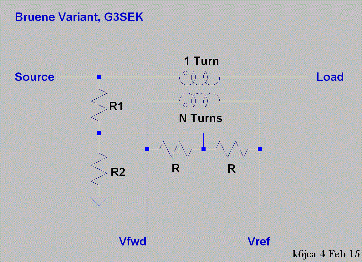
The first is that a resistive voltage divider replaces the capacitive voltage divider.
The second is that the voltage sample from the resistor divider now feeds the junction of two resistors instead of the transformer center-tap.
I'll skip analysis -- the process is no different that what we've done earlier in this post.
Frankly, I don't know if it's better to feed the voltage-sample to the common-point between two resistors, as done above, or to the center-tap of the transformer secondary, as done by ZL1AN. Our concerns are: what is the effect on Directivity, and what is the effect on Frequency Response?
Other Riffs on the Same Theme:
Vc can feed both the resistors and the transformer center-tap. (Any negative effects? I don't know.)

The common point between the two resistors could be tied to ground. But I'm not sure I'd recommend this -- it puts the two resistors in parallel with C2, which means that the frequency response of Vc will no longer be flat. (The secondary of the transformer acts as an auto transformer, and thus, if Vc feeds its center-tap, it will look like a low impedance (i.e. short) to its two ends. Which is to say -- it doesn't act as a common-mode choke when feeding the center-).

Here's another interesting variation, found on G3YNH's website (worth a visit!). A single core is used, but the secondary consists of two windings that are not interconnected. Thus, two voltage dividers are necessary in order to create voltage samples for the two independent windings.

Analysis is similar to the other variants. Voltage and current samples add on the left-hand side. And they subtract on the right-hand side. I don't know what the advantage is to doing it this way, though. But one advantage might be that the transformer's secondary, no longer center-tapped, doesn't act like a "shorting" auto-transformer to Vc's common-mode path to ground. Now, there is some impedance in the path (due to the inductance of each of the secondary coils), but I'm not sure how effective this would be, as it will depend upon the resistance "R" of the two resistors which parallel these coils.
That covers the variants that I've seen that are obviously similar to the ZL1AN topology (and thus will analyze in a similar fashion). I'll introduce below a few more variants that stray a bit further afield (but not by much).
The models presented thus far are in some cases simplified models of the actual circuits. I've left off components that might be related to frequency compensation, or detection, or other functions deemed secondary, because I felt they would detract from understanding the underlying theory of operation. If you're interested in more details, please click on the links I've provided!
As to the positives and negatives for each topology, I wish I had some answers, but I don't. If you have any experience or thoughts on the subject, please feel free to let me know, either via comments to the post or email.
Continuing on...
Bruene Variant, W7EL:
Here's an interesting take on the Bruene Coupler, published by W7EL in the Feb, 1990 issue of QST magazine.
Per the article, this version has +/- 7% accuracy over the range of 1 to 432 MHz. Quite impressive!
At first glance the design looks similar to the Tandem-Match coupler, but it really is a variant on the Bruene topology; the current sample is either added-to, or subtracted-from, the voltage sample. (With the Tandem-Match coupler, it's the voltage sample that is either added-to, or subtracted-from, the current sample).
The two transformers to ground create two voltage samples of the same polarity and whose value is V/N, where V is the voltage on the line.
The "series" transformer samples the line current, I, and its secondary generates a current that is I/N in amplitude.
If "I" is flowing from left-to-right in the diagram below (into the 1-turn primary's "dot"), the secondary current runs from left-to-right (out of the secondary's "dot"). This current creates a positive voltage of amplitude I*51/N across the left-hand resistor and a negative voltage (w.r.t. ground) across the right-hand resistor of amplitude -(I*51/N).
The voltage samples generated by the two voltage-sampling transformers are in series with their respective resistors, and thus Vfwd is the sum of the positive voltage across the left-hand resistor and the positive voltage across left-hand secondary, while Vref is the sum of the negative voltage across the right-hand resistor plus the positive voltage across the right-hand secondary.

The only negative that I can see with respect to the design is that you need to wind 3 transformers!
Bruene Variant, N2PK Power Meter:
N2PK cleverly used the differential inputs of the AD8307 Log Amplifier to do the summing and differencing of the voltage and current samples in his homebrew Power Meter.

That's it for the analysis of Bruene variants! Analysis of the actual Bruene design will follow in Part 2...
Links to my Directional Coupler blog posts:
Notes on the Bruene Coupler, Part 2
Notes on the Bruene Coupler, Part 1
Notes on HF Directional Couplers (Tandem Match)
- I analyzed the Tandem-Match coupler in terms of "lumped" circuit elements, not distributed elements.
- The coupler works by taking a sample of the voltage across the transmission line at a single point and a sample of the current through that point.
- The Tandem-Match Coupler creates both of these samples with transformers.
- The voltage at the "Forward Port" (that we measure on our meter) is calculated by adding the current and voltage samples.
- The voltage at the "Reflected Port" is calculated by subtracting the current and voltage samples.
- The voltage at the "Reflected Port" is 0 when the load is a real resistance equal to the value of the resistors terminating the measurement ports (Forward and Reflected Ports). Thus, the resistor values should be selected to be the same as the characteristic impedance, Zo, of the transmission-line system into which the the coupler is inserted.
- I explained operation of the coupler both in terms of Forward and Reflected waves and also without using waves, instead in terms of only the voltage driving the coupler and the load at its output port.
I'll analyze the original design as well as some of the variants it inspired. Again, I will use lumped-element analysis, and I'll present explanations in terms of forward and reflected waves and also in terms of the voltage being applied to the coupler and the load connected to its output port.
My goal is to present you with an explanation that is understandable -- this will not be a rigorous analysis. So, when possible, I will take advantage of models and assumptions that will simplify the math and hopefully help you grasp the underlying principles.
So here we go! Let's start with the schematic of the Bruene Coupler:
(click on image to enlarge)
There are two capacitive voltage dividers; one is used for generating the Vref voltage, the other is used for the Vfwd voltage. Let's call these the voltage samples, but in fact, they are more than that because of the two diodes connected to them.
Line current passing through the 1-turn primary of a 1:60 turn transformer and induces current in the 60-turn secondary. This current, in turn, is transformed into voltage as it passes through the two 10 ohm resistors. One voltage is positive with respect to ground, the other is negative. These two voltages represent the current sample.
Now the explanation gets a bit tricky. Take a look at the schematic -- we're measuring Vref and Vfwd at the voltage-divider taps. This means that the two caps comprising each voltage-divider aren't simply generating a voltage divided down from the line voltage, they are also involved in adding or subtracting the current-sample voltages, too, so that, when we measure the voltage across either 500 pf cap, it's actually the sum or difference of voltage and current samples.
It wasn't obvious to me how the summing/differencing of voltage and current samples at the voltage-divider nodes was being accomplished. It turns out the diodes linking the voltage-dividers and the current samples play a crucial role -- they are creating a DC voltage at the voltage-divider "tap" to which their Cathodes are connected. But not as series rectifiers -- the diodes instead are serving as "shunt" rectifiers.
The DC voltage they create is a function of the phase and amplitude differences between the voltage and current samples. I'll explain the role these caps and diodes play in more detail as it's interesting, but it's also a a bit complex. So instead let me kick off this post with an analysis of a Bruene variant that isn't quite so daunting.
(I'll get back to Bruene's original circuit, but it will be in another blog post -- look for Part 2!).
And before I get any further into this discussion, let me also make this important point:
I will first look at the Bruene Coupler in terms of Forward and Reflected waves. The Bruene Coupler, being made of "lumped elements" (in the first example below: 2 capacitors, 1 transformer, and 1 resistor), is only looking at the voltage and current present at its output port. It has no idea what the load is, or even how the load is connected to the port. The load might be a resistor or other component simply clipped onto the output connector with test leads, or it might be a length of transmission line with a load (either known or unknown) at its other end.
Irrespective of what the load actually is (transmission line, clipped-on component, or whatever), the Bruene Coupler gives us voltage readings that can be interpreted in terms of Forward and Reflected waves. It is important to remember: these readings should only be interpreted as representing actual Forward and Reflected waves when the Bruene Coupler is connected in a transmission line with the same characteristic impedance, Zo, as the Coupler's designed-for target impedance!
I'll start this analysis assuming the Bruene Coupler is inserted into a transmission line of the designed-for (target) characteristic impedance, Zo. I will follow that with a look at its operation in a non-transmission line environment.
Bruene Coupler Variant, ZL1AN
ZL1AN has written an excellent article explaining a variation on Bruene's original coupler design, and I strongly recommend you take a look at it. Tthe Heathkit HM-102 (and I believe also the Drake W4) used this version of the circuit. I'll simplify the analysis a bit by assuming that the current-sampling is done with an ideal transformer.
Here's ZL1AN's circuit:
(click on image to enlarge)
Let's take this circuit and add a bit more information...
(click on image to enlarge)
In the image above:
- "V" is the voltage across the transmission line at our "point" of measurement. We will assume that the voltages are the same at the input and output ports of the coupler -- there is no drop through the coupler.
- "I" is the current on the transmission line through that point.
- I've replaced the resistor load (of resistance "R" ohms) across the transformer secondary with two series resistors of value R/2.
- The voltage at the junction of these two resistors is Vc, because the voltage at the center-tap of the transformer is Vc, and these two resistor form a divide-by-2 voltage divider across the secondary that essentially places their junction at the same voltage as the center-tap.
- Current "I" through the transformer primary induces a current "Is" in the secondary.
- Is = I/(2*N), and it flows in the opposite direction of I (per the transformer "dots" that I've shown).
- We assume that no current flows out either the Vfwd or Vref measurement ports.
- Therefore there is no load on our capacitive divider's voltage "Vc" (that is, there isn't another path from Vc to ground that parallels the path through C2).
- Therefore the voltage at Vc is:
Vc = V*(1/(jw*C2)) / ((1/(jw*C1))+(1/(jw*C2)))
If 1/(jw*C1) >> 1/(jw*C2), this simplifies to: Vc = V*C1/C2
(click on image to enlarge)
Vfwd and Vref are easily calculate from the series addition of Vc and the appropriate voltage generated by the current sample:
Vfwd = Vc + Is*R/2
Vref = Vc - Is*R/2
Substituting in our equations for V and Is, we get:
Vfwd = V*(C1/C2) + I*R/(4*N) (equation 1)
Vref = V*(C1/C2) - I*R/(4*N) (equation 2)
Analysis Using Forward and Reflected Waves
Let's first analyze this circuit in terms of Forward and Reflected waves passing through our coupler.
The Forward and Reflected waves each have a voltage and a current: Vf and If are the voltage and current of the forward wave, and Vr and Ir are the voltage and current of the reflected (or reverse) wave.
(click on image to enlarge)
The total voltage on the line, V, at any point is the sum of Vf and Vr at that point.
V = Vf + Vr
And the total current on the line, I, at any point is the difference of If and Ir at that point (they subtract because Ir is flowing in the opposite direction of If).
I = If - Ir
We also know:
If = Vf/Zo
Ir = Vr/Zo
Where Zo is the characteristic impedance of the transmission line.
So, substituting and rearranging, equations 1 and 2 become:
Vfwd = (Vf+Vr)*(C1/C2) + (Vf/Zo - Vr/Zo)*R/(4*N)
Vref = (Vf+Vr)*(C1/C2) - (Vf/Zo - Vr/Zo)*R/(4*N)
Regrouping terms:
Vfwd = Vf*((C1/C2) + R/(4*N*Zo)) + Vr*((C1/C2) - R/(4*N*Zo))
Vref = Vf*((C1/C2) - R/(4*N*Zo)) + Vr*((C1/C2) + R/(4*N*Zo))
Notice what happens if we select our components such that they meet the following requirement:
C1/C2 = R/(4*N*Zo) = K (equation 3)
The two equations reduce down to:
Vfwd = Vf*2*K
Vref = Vr*2*K
So, if we select C1, C2, R, and N such that the satisfy the relationship above, then the voltage we measure at Vfwd is solely related Vf, the voltage of the Forward wave, and the voltage we measure at Vref is solely related to Vr, the voltage of the Reflected (or Reverse) wave!
Analysis in a non-Transmission Line Environment:
It's instructional to analyze the operation of the directional coupler just in terms of the components themselves, the voltage applied to the coupler, and the load at its output port without using the concepts of waves. After all, the coupler consists of lumped-elements, so there's no real reason to think of its operation in terms of waves.
So let's draw our circuit like this, where V is the voltage source driving the input of the Bruene Coupler and Zload is connected to its output.
We'll use the same assumptions that we used above. Therefore equations 1 and 2 still hold:
Vfwd = V*(C1/C2) + I*R/(4*N) (equation 1)
Vref = V*(C1/C2) - I*R/(4*N) (equation 2)
This time, rather than expressing V and I in terms of waves, we will note that "I" is simply "V" divided by Zload:
I = V/Zload
If we substitute this equation into equations 1 and 2, we get:
Vfwd = V*((C1/C2) + R/(4*N*Zload)) (equation 4)
Vref = V*((C1/C2) - R/(4*N*Zload)) (equation
5)
Now let's take equation 3:
C1/C2 = R/(4*N*Zo) = K (equation 3)
Let's take that second half:
R/(4*N*Zo) = K
And rearrange it:
R/(4*N) = K*Zo (equation 6)
Where Zo can be considered to be our "Target" impedance. Usually this is selected to be the impedance of the transmission line, but it needn't be.
Now let's plug equations 3 and 6 into 4 and 5 and reduce. We get:
Vfwd = V*K*(Zload + Zo)/Zload
Vref = V*K*(Zload - Zo)/Zload
Well, these are interesting equations. If Zload equals our target Zo that we selected our components for (e.g. 50 ohms), then Vfwd = V*2*K and Vref = 0.
We could use these equations as they are, but note what happens if we take these two voltages and divide one into the other. We get something that ought to look familiar:
Vref/Vfwd = (Zload - Zo) / (Zload + Zo)
Which is the definition of Reflection Coefficient!
So we can use the voltages measured at Vref and Vfwd to determine an impedance relationship (i.e. imbalance) between the actual Zload and coupler's "target" impedance of Zo. And this impedance relationship is exactly the same as the Reflection Coefficient.
SWR is easily calculated from the Reflection Coefficient:
SWR = (1 + |Reflection Coefficient|) / (1 - |Reflection Coefficient|)
Note that, although SWR implies the presence of Forward and Reflected waves, we have no guarantee that what we measure (or calculate) to be SWR or Forward/Reflected power is actually what is happening in our system. I'll quote G3YNH:
"[The bridge] can only infer the existence of reflected power from the difference between the actual load impedance and the target load impedance. To understand this point, consider an SWR bridge designed to balance when the load is 50+j0Ω. If we connect this bridge directly to a 100Ω load resistor, it will declare an SWR of 2:1. The resistor is not reactive however, and so will absorb all of the power delivered to it and reflect none. The 2:1 SWR reading is only true when the bridge sees an impedance magnitude of 100Ω (or 25Ω) at the input to a 50Ω transmission line. The bridge is just an impedance bridge, it has no special psychic powers, and its readings are only true when it is inserted into a line having the same characteristic resistance."So, summing up:
It should be evident from the above analysis that we don't need to rely on the concepts and Forward and Reflected waves to understand how the Bruene coupler operates.
Our typical "Bruene" SWR meter is really just calculating a relationship between the load at its output port (Zload) and its own design parameters (i.e. C1/C2 = R/(4*N*Zo) = K). And this relationship is equivalent to the Reflection Coefficient if "Zo" in the relationship: "C1/C2 = R/(4*N*Zo) = K" is the same as the characteristic impedance of the transmission line, should the coupler be connected to a transmission line.
It's important to note that Zload could be a load connected directly to the coupler's "OUT" port with a couple of wires, or it could be the impedance "presented" to the port by a long length of transmission line (an impedance determined, at that point, by the interaction of the Forward and Reflected waves).
The coupler doesn't care "how" the load is connected to its OUT port. It's just looking at the voltage across the OUT port and the current through the OUT port. It doesn't know anything else about the load except for this voltage and current relationship at its OUT port. For example, if the OUT port happens to be connected to a transmission line, the coupler has no knowledge of the line's Zo. It doesn't even know if there's a transmission line attached, nor that the impedance it sees at its OUT port might be due to the interaction of Forward and Reflected waves.
For this reason, never assume that the meter reading is the actual Reflection Coefficient, Γ, or that the SWR reading is the actual SWR reading of the line. It might not be. We are really just measuring the relationship between Zload (as it appears at the OUT port) and the design parameters of the coupler. Only if the "Zo" in the design relationship "C1/C2 = R/(4*N*Zo) = K" equals the actual characteristic impedance, Zo, of the transmission line would we truly be measuring the Reflection Coefficient.
And on that note, I'll end this non-Transmission Line analysis!
Frequency Insensitivity:
If you refer back to the equations for Vfwd and Vref, you should notice something interesting: there are no j*w terms (where omega (w) = 2*pi*frequency). This means that the voltage-divider voltage, Vc, and the voltage generated by the current-sample via the transformer are both constant over frequency.
Of course, in the real world nothing is perfect and there will be effects due to strays and parasitics. Never the less, if designed correctly (to deal with strays), the frequency response should be flat over a broad range of frequencies.
Which leads to an interesting observation: If the voltage divider is independent of frequency, why use capacitors?
Well, one doesn't need to use caps, we could just as easily use inductors (whose "jw" terms will cancel), or even resistors!
Which leads me to another variant of the Bruene coupler, which can be found in G3SEK's "In Practice" column in the September, 2002 issue of Radcom...
Bruene Coupler Variants, G3SEK:
One of the coupler's described in G3SEK's column looks very similar to the coupler described by ZL1AN, but there are a few differences:
The first is that a resistive voltage divider replaces the capacitive voltage divider.
The second is that the voltage sample from the resistor divider now feeds the junction of two resistors instead of the transformer center-tap.
I'll skip analysis -- the process is no different that what we've done earlier in this post.
Frankly, I don't know if it's better to feed the voltage-sample to the common-point between two resistors, as done above, or to the center-tap of the transformer secondary, as done by ZL1AN. Our concerns are: what is the effect on Directivity, and what is the effect on Frequency Response?
Other Riffs on the Same Theme:
Vc can feed both the resistors and the transformer center-tap. (Any negative effects? I don't know.)
The common point between the two resistors could be tied to ground. But I'm not sure I'd recommend this -- it puts the two resistors in parallel with C2, which means that the frequency response of Vc will no longer be flat. (The secondary of the transformer acts as an auto transformer, and thus, if Vc feeds its center-tap, it will look like a low impedance (i.e. short) to its two ends. Which is to say -- it doesn't act as a common-mode choke when feeding the center-).
Here's another interesting variation, found on G3YNH's website (worth a visit!). A single core is used, but the secondary consists of two windings that are not interconnected. Thus, two voltage dividers are necessary in order to create voltage samples for the two independent windings.
Analysis is similar to the other variants. Voltage and current samples add on the left-hand side. And they subtract on the right-hand side. I don't know what the advantage is to doing it this way, though. But one advantage might be that the transformer's secondary, no longer center-tapped, doesn't act like a "shorting" auto-transformer to Vc's common-mode path to ground. Now, there is some impedance in the path (due to the inductance of each of the secondary coils), but I'm not sure how effective this would be, as it will depend upon the resistance "R" of the two resistors which parallel these coils.
That covers the variants that I've seen that are obviously similar to the ZL1AN topology (and thus will analyze in a similar fashion). I'll introduce below a few more variants that stray a bit further afield (but not by much).
The models presented thus far are in some cases simplified models of the actual circuits. I've left off components that might be related to frequency compensation, or detection, or other functions deemed secondary, because I felt they would detract from understanding the underlying theory of operation. If you're interested in more details, please click on the links I've provided!
As to the positives and negatives for each topology, I wish I had some answers, but I don't. If you have any experience or thoughts on the subject, please feel free to let me know, either via comments to the post or email.
Continuing on...
Bruene Variant, W7EL:
Here's an interesting take on the Bruene Coupler, published by W7EL in the Feb, 1990 issue of QST magazine.
Per the article, this version has +/- 7% accuracy over the range of 1 to 432 MHz. Quite impressive!
At first glance the design looks similar to the Tandem-Match coupler, but it really is a variant on the Bruene topology; the current sample is either added-to, or subtracted-from, the voltage sample. (With the Tandem-Match coupler, it's the voltage sample that is either added-to, or subtracted-from, the current sample).
The two transformers to ground create two voltage samples of the same polarity and whose value is V/N, where V is the voltage on the line.
The "series" transformer samples the line current, I, and its secondary generates a current that is I/N in amplitude.
If "I" is flowing from left-to-right in the diagram below (into the 1-turn primary's "dot"), the secondary current runs from left-to-right (out of the secondary's "dot"). This current creates a positive voltage of amplitude I*51/N across the left-hand resistor and a negative voltage (w.r.t. ground) across the right-hand resistor of amplitude -(I*51/N).
The voltage samples generated by the two voltage-sampling transformers are in series with their respective resistors, and thus Vfwd is the sum of the positive voltage across the left-hand resistor and the positive voltage across left-hand secondary, while Vref is the sum of the negative voltage across the right-hand resistor plus the positive voltage across the right-hand secondary.
The only negative that I can see with respect to the design is that you need to wind 3 transformers!
Bruene Variant, N2PK Power Meter:
N2PK cleverly used the differential inputs of the AD8307 Log Amplifier to do the summing and differencing of the voltage and current samples in his homebrew Power Meter.
That's it for the analysis of Bruene variants! Analysis of the actual Bruene design will follow in Part 2...
Links to my Directional Coupler blog posts:
Notes on the Bruene Coupler, Part 2
Notes on the Bruene Coupler, Part 1
Notes on HF Directional Couplers (Tandem Match)
Building an HF Directional Coupler
Notes on the Bird Wattmeter
Notes on the Monimatch
Notes on the Twin-lead "Twin-Lamp" SWR Indicator
Calculating Flux Density in Tandem-Match Transformers
And some related links from my Auto-Tuner and my HF PA posts:
Auto Tuner, Part 5: Directional Coupler Design
Auto Tuner, Part 6: Notes on Match Detection
Auto Tuner, Part 8: The Build, Phase 2 (Integration of Match Detection)
HF PA, Part 5: T/R Switching and Output Directional Coupler
Bruene Coupler References:
Bruene, Warren, "An Inside Picture of Directional Wattmeters," QST, Apr., 1959. Includes both a good explanation of the Monimatch operation and a design for a directional wattmeter whose directional coupler topology would later be known as the "Bruene Coupler."
Collins 302C-3 Directional Wattmeter, PDF Manual containing schematic.
Rush, James, Jr., "The Mini-Mono-Monimatch," QST, Mar., 1965. Although called a Monimatch in the title, the design actually is more similar to Bruene's directional coupler.
Bold, Gary, ZL1AN, "The Bruene Directional Coupler and Transmission Lines," PDF. This PDF gives an excellent explanation of the Bruene Coupler.
Kiciak, Paul, N2PK, "An HF In-Line Return Loss and Power Meter," PDF. Constructions details of a power meter using a Bruene Coupler. Contains an explanation by the other of why he prefers the Bruene coupler of the Tandem-Match Coupler. Also interesting because the author separates the voltage-sampler from the current sampler and uses the differential inputs of an AD8307 to do the required addition (or subtraction) to get FWD and REF voltages.
(This web page could be useful for understanding the sampling method used in the N2PK meter: http://www.g3ynh.info/zdocs/bridges/magdiff/part1.html )
Lewallen, Roy, W7EL, "A Simple and Accurate QRP Directional Wattmeter," QST, Feb, 1990, PDF. Interesting variant of the Bruene coupler. Roy uses two transformers for the voltage sample in lieu of capacitor voltage dividers.
White, Ian, G3SEK, "Inside a Directional Wattmeter," RadCom, Sept., 2002, PDF. Discussion and a bit of analysis of Bruene coupler. Includes Bruene's phase-relationship diagrams.
http://www.g3ynh.info/zdocs/bridges/reflectom/part1.html interesting analysis
http://www.g3ynh.info/circuits/Diode_det.pdf Diode detectors -- includes some info on shunt detectors, which is what Bruene's design uses.
Other references of generally interest:
http://www.g3ynh.info/zdocs/bridges/Xformers/part_1.html great discussion on current-transformers for directional coupler applications
http://www.g3ynh.info/zdocs/bridges/Xformers/part_2.html Part 2 of current-transformers
http://www.g3ynh.info/zdocs/bridges/Xformers/part_3.html And part 3, the last part, of current-transformers
http://www.g3ynh.info/zdocs/bridges/index.html Indexes numerous topics. Lots of great info to be found here!
http://www.richtek.com/assets/AppNote/AN008_EN/AN008_EN.jsp Common-Mode choke model
Final Caveats:
As always, I might have made a mistake in my equations, assumptions, or interpretations. If you see anything you believe to be in error, or if anything is confusing, please feel free to contact me.
Notes on the Bird Wattmeter
Notes on the Monimatch
Notes on the Twin-lead "Twin-Lamp" SWR Indicator
Calculating Flux Density in Tandem-Match Transformers
And some related links from my Auto-Tuner and my HF PA posts:
Auto Tuner, Part 5: Directional Coupler Design
Auto Tuner, Part 6: Notes on Match Detection
Auto Tuner, Part 8: The Build, Phase 2 (Integration of Match Detection)
HF PA, Part 5: T/R Switching and Output Directional Coupler
Bruene Coupler References:
Bruene, Warren, "An Inside Picture of Directional Wattmeters," QST, Apr., 1959. Includes both a good explanation of the Monimatch operation and a design for a directional wattmeter whose directional coupler topology would later be known as the "Bruene Coupler."
Collins 302C-3 Directional Wattmeter, PDF Manual containing schematic.
Rush, James, Jr., "The Mini-Mono-Monimatch," QST, Mar., 1965. Although called a Monimatch in the title, the design actually is more similar to Bruene's directional coupler.
Bold, Gary, ZL1AN, "The Bruene Directional Coupler and Transmission Lines," PDF. This PDF gives an excellent explanation of the Bruene Coupler.
Kiciak, Paul, N2PK, "An HF In-Line Return Loss and Power Meter," PDF. Constructions details of a power meter using a Bruene Coupler. Contains an explanation by the other of why he prefers the Bruene coupler of the Tandem-Match Coupler. Also interesting because the author separates the voltage-sampler from the current sampler and uses the differential inputs of an AD8307 to do the required addition (or subtraction) to get FWD and REF voltages.
(This web page could be useful for understanding the sampling method used in the N2PK meter: http://www.g3ynh.info/zdocs/bridges/magdiff/part1.html )
Lewallen, Roy, W7EL, "A Simple and Accurate QRP Directional Wattmeter," QST, Feb, 1990, PDF. Interesting variant of the Bruene coupler. Roy uses two transformers for the voltage sample in lieu of capacitor voltage dividers.
White, Ian, G3SEK, "Inside a Directional Wattmeter," RadCom, Sept., 2002, PDF. Discussion and a bit of analysis of Bruene coupler. Includes Bruene's phase-relationship diagrams.
http://www.g3ynh.info/zdocs/bridges/reflectom/part1.html interesting analysis
http://www.g3ynh.info/circuits/Diode_det.pdf Diode detectors -- includes some info on shunt detectors, which is what Bruene's design uses.
Other references of generally interest:
http://www.g3ynh.info/zdocs/bridges/Xformers/part_1.html great discussion on current-transformers for directional coupler applications
http://www.g3ynh.info/zdocs/bridges/Xformers/part_2.html Part 2 of current-transformers
http://www.g3ynh.info/zdocs/bridges/Xformers/part_3.html And part 3, the last part, of current-transformers
http://www.g3ynh.info/zdocs/bridges/index.html Indexes numerous topics. Lots of great info to be found here!
http://www.richtek.com/assets/AppNote/AN008_EN/AN008_EN.jsp Common-Mode choke model
Final Caveats:
As always, I might have made a mistake in my equations, assumptions, or interpretations. If you see anything you believe to be in error, or if anything is confusing, please feel free to contact me.


