A 20 through 10 meter 43-foot Vertical Doublet

I'm not a contester, but a good contest always provides an opportunity for working DX, even for those of us who aren't running kilowatts and stacked yagis.

Next weekend (March 7th, 2015) is the ARRL's DX Contest (Phone).  I'll be up at the "portable 6" location during that weekend, and I would normally use my full-wave 80 meter loop that I have up there.  But the loop, being an oddball shape due to support-tree locations, not too surprisingly has oddball patterns.  For example, here's its azimuth plot on 10 meters:

Some nice gain in some directions.  In others...not so much.  Although it hasn't been a big issue working DX during contests, I have noticed the nulls in the pattern.  So I thought...why not try something else, for comparison?

Given the short time frame between antenna installation and actual contest, my design constraints were:

1. Easy to install.
2. 20, 15, and 10 meter operation (and preferably the WARC bands, too).
3. There's no tower on site, so pattern should be omnidirectional (to fill in the existing loop's holes).
4. Some gain, whenever possible (maximize gain on 10 meters, if possible).
5. Temporary installation, so must disassemble easily.

Horizontal antennas (e.g. dipoles, yagi's, etc.) were pretty much precluded due to their directionality -- I have no way to turn them.  And installing multiple dipoles seemed problematic due to support-tree locations.

So I started looking at verticals.

Ground mounted verticals all seemed to have either fairly high-angled radiation patterns or low gain.  But because there are some very high trees at the QTH here (100 feet, plus), why not raise a vertical up and get it as far off the ground as I could?  Of course, it would then no longer be a quarter-wave vertical, but a dipole of some sort.

I also wanted to try to maximize the gain on 10 and 15 meters with low angles of radiation.  So I started playing around with vertically mounted dipoles (i.e. doublets), varying their heights and lengths using EZNEC, the antenna simulation program.

43 feet (21.5 feet on each side of the feedpoint) seemed like a great length.  10 meter gain peaked at about 6.9 dBi at 7 degrees elevation (a very nice low angle!), compared to other doublet lengths I tested (which were from 28 to 53 feet, in 5 foot increments).

Here are the EZNEC windows...

(click on image to enlarge)

Note that the source is placed in the center of the antenna.  When I later use EZNEC to calculate SWR, this will be the point at which it calculates SWR:  at the antenna itself.

 (click on image to enlarge)

 (click on image to enlarge)

 ...and EZNEC plots (click on images to enlarge):

 

6.9 dBi at 7 degrees.  Not bad!

Being 43 feet long, the antenna itself was non-resonant on all of the ham frequencies, so it would have a high SWR. Clearly, it should be feed with ladder-line (rather than coax) to minimize SWR-related power loss.  But how long should the line be?

There's actually a science to determining feed line length (although sometimes you have to go with what you have on hand, as I did with the feedline to my 80 meter loop).  Depending upon the antenna, certain feedline lengths will produce low SWRs on multiple ham bands.  The G5RV (designed by Louis Varney in 1946) is probably the best known example of this type of multiband antenna.  The ZS6BKW doublet is another example, as is W5DXP's no-tuner antenna.

So what's the science?

The goal is to get the SWR in the ham bands (as seen by the antenna turner) down to a low enough level to allow the tuner to get it the rest of the way down to 1:1 (hopefully without too much power lost in the tuner).

Because the antenna itself is non-resonant on the ham bands, its impedance (and thus SWR) at ham-radio frequencies will be high.  Coax can have significant loss at higher frequencies (when operating with a high SWR), plus it's fairly heavy, which makes it a poor choice to feed my vertical-doublet suspended between trees.  Ladder-line has lower loss and is lighter weight -- it's a much better choice, and the fact that its characteristic impedance is much higher than 50 ohms works in our advantage, too.

Let's see how.  If I were feeding the doublet with 50 ohm coax, EZNEC calculates that the SWR at 28.5 MHz would be 80.8:1 (!!!).  With 400 ohm ladder line this becomes a more reasonable (but still high) 12.3:1.

So we are already ahead, compared to 50 ohms, but 12.3:1 is still pretty high.  I'd like my tuner to see something lower.  And I can do this by intelligently selecting the length of 400 ohm ladder line.  I'll use the Smith chart below to demonstrate how:

(click on image to enlarge)

First, a few points about Smith Charts...

It's important to understand that the Smith Chart can be thought of as an overlay over a plot of the Reflection Coefficient (referenced to a Zo of the user's preference).  The reflection coefficient (also known as Γ (the Greek Gamma)) can be expressed either as a complex quantity using Cartesian coordinates (x-axis = real component, y-axis = imaginary (or reactive) component) or as a polar coordinate.  In the image above the point I've selected is at 0.5355 - j0.6, or, expressed in polar coordinates, 0.85 magnitude, -51 degrees; both are equivalent.

In the Smith Chart above, the outer circle designates a reflection coefficient of magnitude 1 (infinite SWR).  At the "0 degree" point on this outer circle (x-axis, right-hand side), the coordinates can be expressed either 1 + j0 (x,y axis) or as 1, 0° (polar), both are equivalent.  This point corresponds to a load of infinite resistance and no reactance.  That is, an unconnected transmission line.

At 180 degrees the coordinates are -1 + j0 (x,y axis) or 1, 180° (polar).  This point represents a load of 0 ohms resistive and no reactance.   In other words, a short at the end of the transmission line.

At 90 and -90 degrees on the outer circle the coordinated can be written either as 0+j (or 0, 90 degrees), or 0-j (or 0, -90 degree), respectively.  So the values along the y-axis are solely reactive with no resistance.

The center of the Smith Chart is our reference Characteristic Impedance (Zo) used to calculate the reflection coefficient, Γ.  In this example, Zo is the impedance of the ladder line I'm using (400 ohms:  JSC 1315).  And at this center point the reflection coefficient is 0; that is, a perfect match to 400 ohms.

I've also added two interesting SWR circles to the chart.  One is for an SWR of 4:1.  It intersects the left-hand x axis at 100+j0 (i.e. 100 ohms, resistive).

The next is an SWR circle of 16:1 intersects the circle at 25 ohms, resistive.

I chose these circles for a specific purpose.  First, the doublet's SWRs that EZNEC calculates at 14.2, 18.1, 21.3, 24.96, and 28.5 MHz are bounded between the inner 4:1 and outer 16:1 SWR circles.

And second (and perhaps the most important), the impedance values where these circles intersect the left-hand x axis lie between 25 and 100 ohms, resistive  -- that is, these SWR circles, if the proper lengths of transmission line are chosen, will result in an SWR of lower than 2:1 (referenced to 50 ohms) at the "transmitter" end to the transmission line.  And it is to this end of the ladder line, now presenting a low SWR relative to 50 ohms, that I can connect my 50 ohm tuner, SWR meter, and transmitter.

So how long does the ladder line need to be to transform the antenna's impedance to the lower, friendlier impedance on the left-hand x axis?

It's actually easy to calculate.  First, recognize that EZNEC, when it calculates SWR, returns the reflection coefficient along with the SWR.  For example, for a Zo of 400 ohms at 28.5 MHz, EZNEC expresses the reflection coefficient of my vertical doublet  in both Cartesian and polar coordinates: 0.5355-j0.66 and magnitude 0.85, angle of -51°, respectively.

(click on image to enlarge)

You can see this point on the Smith Chart below.  I've also shown its SWR circle (12.3:1).  Note that it intersects the left-hand x axis at 32.5 ohms, which would result in an SWR of 1.5:1 in a 50 ohms system.

(click on image to enlarge)

Okay, a quick Smith Chart digression:  if a transmission line is lossless (they aren't but for the moment we will assume they are), as we increase the length of the transmission line, we'll move clockwise around a Smith Chart's circle of constant SWR.  For example, if the transmission line is lengthened by (λ/4)*Vf (where λ is wavelength and Vf is the transmission line's Velocity Factor), we will rotate 180 degrees around the SWR circle.  And if the transmission line is lengthened by (λ/2)*Vf (that is, a half-wavelength), we will rotate through a full 360 degrees and wind up where we started.

Now back to the problem.  The angle of the reflection coefficient, at the antenna, is -51 degrees, and it lies on the "SWR = 12.3" circle. To get to 32.5 ohms, resistive, the ladder line needs to be long enough to rotate the angle of the reflection coefficient by an additional 129 degrees clockwise (actually, 129.05 degrees).  So how long should the line be to achieve this rotation?

Knowing that 180 degrees of rotation equals a change of length of (λ/4)*Vf (see the earlier paragraph), I can set up a simple ratio, where x is the length I'm solving for:

Angle-to-rotate/180 = x / ((λ / 4) * Vf)

Rearranging to solve for x:

x = (Angle-to-rotate / 180) * ((λ / 4) * Vf)

We know that the "angle-to-rotate" is 129 degrees.  The solution is straight forward, but for one small snag specific to my JSC ladder line:  The JSC website does not specify the Velocity Factor of its 1315 ladder line.  Well, all is not lost; I can take a swag at it.  If I look at Wireman 522 ladder line (also with 16 AWG stranded wire), its Vf is 0.91.  Googling shows other ladder line with a Vf of  0.85.  Let me take the average of these two, 0.88, as the Vf.  Using this value, the result for x is:

x = 5.45 feet

So if I feed the antenna with 5.45 feet of 400 ohm ladder line, I should see 32.5 ohms at the ladder line's other end (when measured at 28.5 MHz) if, as I hope, the Vf is 0.88..  If I then add ladder line in lengths that are a multiple of (λ/2)*Vf (in this example, 15.19 feet), the resulting impedance that I measure at the end of the transmission line will still be 32.5 ohms.

I've set up an Excel spreadsheet to easily calculate the lengths of transmission line that intersect the left-hand x axis of the Smith Chart.  You'll see two different sets of calculations below.  One is for a Vf of 0.85, the other is for a Vf of 0.88.

(click on image to enlarge)

Notice the groupings in the cells with common colors.  If the ladder line length is about 51 feet (for a Vf of 0.88), we'll intersect the Smith Chart's left axis (or be close to it) for 20, 15, and 10 meters.  Perfect for my contest application!

Except...51 feet is too short to reach the house.  Nix that.

The next grouping is at about 83 feet of line.  Looks pretty good on 20, 17, and 10 meters, but not so much on 15.  (I actually tried this length.  If I compared the 80 meter full-wave loop to the vertical doublet, background noise was roughly equivalent between the two antennas on all bands except on 15 meters, where background noise was way down on the vertical doublet (ditto with signals), indicating to me it was performing poorly.)

Well, for the contest I really want to have 15 meters, too.  So nix 83 feet.

So on to about 112 feet (there's probably plus/minus a foot or two of measurement error on my part).  Hook it up -- sounds pretty good!  15 meters is alive again.  And Japan coming in stronger on the doublet than on the 80 meter full-wave loop.  A good sign!

Let's measure SWR Minima, scanning from 13 MHz to 30 MHz with an MFJ-259B SWR Analyzer:

(click on image to enlarge)

SWRs look good!  A little bit high on 17 meters, but that's to be expected if we look at the values in the earlier table.  Its preferred transmission-line length is an outlier compared to the other frequencies, and wants to be shorter.

Notes on installation:

Raising this antenna was a one-man effort.  All in all, it went well.  Not difficult, but definitely time consuming.  Here's the antenna, finally up:

(click on image to enlarge)

(Actually, it's about 43 feet from the lower insulator to ground, not 45).

All support lines use 3/16 inch dacron polyester rope, launched into trees using my pneumatic antenna launcher.

Reeling in 3/16 inch dacron polyester rope up and over a tree using the 30 lb test line on my launcher really felt like I was pushing it, so I decided to go to an intermediary step and use some flourescent-yellow string I'd purchased at some time in the distant past from the hardware store.  So now I'd shoot my 30 lb test line over the tree, then attaching the string to its far end and reel it in.  When I'd gotten the string back to the reel I'd then tie the 3/16" Dacron rope to its end and pull the rope up and over.

At the far end, I made a simple jig for unspooling using about a three foot length of threaded rod to hold spools of rope (or the string).

I discovered that reeling in the string by hand was much too slow, so I made a quick fixture with a drill to speed things up:

I hung the ladder line in loose coils on a rope under the eaves to keep it off the ground.  (If the trees had been farther from the house, I probably could have skipped this step.)

I installed a Common-Mode choke (a.k.a current-mode balun) at the point where my 16 feet of 50 ohm coax emerges from the shack and connects to the 400 ohm ladder line.

I made the CM choke by wrapping 11 turns of RG-142 around two FT240-61 cores, with the short end of its coax connected to the ladder line.

I did a quick check of its impedance by measuring S21 from BNC-shield at one end of the coax to the BNC-shield at the other end (because this inductance is, essentially, the "leakage path" around the CM choke (a good reference:  W7EL balun)).  Here's a photo of the test setup:

After first normalizing S21 by connecting to a long wire between the two red clips above and, well, normalizing the reading, I measured S21 of the CM choke:

Horizontal divisions are every 3 MHz from 0 MHz.  Vertical divisions are 10 dB per.  So that's about 24 dB of loss at 30 MHz, referenced to 50 ohms.

(Note -- I could have used S11, too, to measure impedance of the coiled cable.)

How effective will this choke actually be?  Well, it depends upon the common-mode impedance that it sees at its terminals, and I don't know what this is.  One quick test would be to measure the currents on the ladder line just after the choke.  If the choke is doing its job, these currents should be equal.

In other words -- a test for the future, after I build a current probe!

(And I'll add, regarding where the choke should be in the line -- it should be placed where the common-mode impedance that it sees is low, because it won't attenuate the common-mode signal much if the common-mode load it sees is high.  If I assume that the common-mode impedance, at the antenna itself (relative to ground far below it) is high, then this implies to me that the choke should be placed on an odd-multiple of  λ/4 back from the antenna (i.e. a low-impedance common-mode point).  One potential issue in determining this position, though:  because the signal is common-mode, I doubt the common-mode velocity factor on the transmission line is the same as the differential velocity factor (which is 0.88, or so).  I don't know what it is, and  I'd be interested to hear others' thoughts on this topic).


Final Thoughts...

This design shows that it's possible to design an antenna with a fixed feedline length that will perform on multiple ham bands without a tuner.  But in this example the feedline needs to be about 112 feet in length.

This length, if we assume feedline characteristics similar to Wireman 552 ladder line (it also has 16 AWG stranded wire, like the JSC ladder line I'm using) has a loss of about 1.5 dB on 10 meters.  Not a lot, but...could we make this less?

Also, 112 feet is a lot of ladder line, much more than I actually need in my application to get from antenna to shack (as you could see in the photo above, with the ladder line coiled in loops along the side of the house).  Definitely a negative on the wife/girlfriend acceptance factor!

And one more thing, SWR isn't great on 17 meters.  So, although close, we haven't exactly hit the target.

If I were to make this antenna permanent, I would actually change how I feed and tune the doublet.  I'd still use ladder line to the antenna itself (in fact, I'd be tempted to make open-wire ladder line to reduce loss/detuning when the line is wet), but I'd keep the run of ladder line short -- just long enough to reach my short length of 50 ohm coax that runs through the house wall from the shack to the outside.

At this junction between coax and ladder line I'd add way to remotely (from the shack) insert, in series between the ladder line and the coax, 1, 2, 4, and/or 8 foot additional lengths of ladder line.  This would let me selectively add a delta to the length of the ladder line from 0 feet to 15 feet, in 1 foot increments, allowing me to tune the length of the feedline for minimum SWR (note that 15 feet is very close to a quarter-wavelength on 20 meters, assuming a Vf of about 0.88)


Resources:

EZNEC

K6JCA Antenna Launcher

JSC Ladder Line

Wireman Ladder Line

Wireman Transmission Line Loss Calculator

W7EL Balun Discussion

Smith V3.10 Smith Chart Program


Standard Caveat:

I easily could have made a mistake in the above posting.  If anything looks wrong or is unclear, please let me know.

Also -- the antenna and transmission line were hastily designed  -- there might be lengths of antenna and/or line that are better suited -- I did not do an exhaustive analysis.  Let me know if you have thoughts on this.

Also, use common sense when installing antennas.  Beware of power lines, and, when shooting lines into trees, keep in mind that free-falling objects could drop on your head (or car!) from above.

Improved Pneumatic Antenna Launcher

About four years ago I built a pneumatic antenna launcher that launched small tennis balls into trees for raising wire antennas.  You can find that earlier post >>here<<.

Recently a friend sent me a link to KR4LO's "Air Boss" Antenna Launcher which uses small 2 oz. "egg sinkers" in lieu of tennis balls.  The Air Boss looks like a well thought out design with great range, and for the price, an excellent deal.

But I already had a launcher that I'd built.  It got me thinking, though...could I modify mine to use the same approach?

Yes, I could.  And I did.  Here's the new design...

The barrel is now a 3 foot length of 3/4 inch diameter schedule 80 grey plastic pipe (threaded at both ends), cut down to about 30 inches (explained below).

My first iteration used white 3/4" diameter PVC pipe for the barrel (1/2" was too narrow), but its inner diameter was slightly too large -- too much air was escaping around the sides of the 2 oz. egg sinker I was using as a weight, compromising its range.  I had to wrap about 7 turns of masking tape around the "waist" of the sinker to bulk it out enough to get a good seal in the pipe (the sinker was still loose inside the barrel, but not too loose).

Compared to the white PVC pipe, the grey pipe has a slightly narrower inner diameter (and it seems stiffer, too -- less likely to bend).  So the egg sinker fits into it better, but I still add about 2 turns of masking tape around the waist of the egg sinkers, but this additional bulking-out might not be needed.

The barrel attaches to a 3/4 inch PVC ball valve (threaded, female connections), so, for storage, it's very easy to unscrew the barrel from the air-chamber/valve assembly.  Note:  my original design used a 1/2 inch ball valve.  This meant that I had to adapt the threaded 3/4" threaded pipe to the 1/2" ball valve.  Which I did.  Unfortunately, during testing I snapped off one of the glue joints near that valve.  Rather than rebuild it with the same 1/2" valve, I thought it better to use a valve that could mate directly with the barrel, without adapters.

This new ball valve is a bit stiffer to turn than my original one.  I was worried that this meant I couldn't turn it as fast, and therefore the "explosion" of air when I opened it wouldn't be as powerful.

I tried lubricating the ball with "Faucet and Valve" grease, but this didn't seem to have any effect.  So I instead jury-rigged a handle-extender with a piece of scrap kindling and a hose clamp:

Not elegant, but it seems to work.

The reel is inexpensive, purchased at Walmart.  The reel came with a cheap no-name, no-spec line pre-installed.  I removed this line and installed in its place 30 lb. test "Spiderwire" braid (about 125 yards).

The fishing reel is attached to the barrel with a couple of hose clamps.

The fishing weights are 2 oz. egg sinkers (I picked mine up at Walmart).  I didn't want the fishing leader to pass on the outside of the sinker, so it runs only inside the sinker, with lead split-shot clamped on the leader at either end to keep the sinker from moving around:

One thing I've learned with antenna launchers, be they sling-shot, pneumatic, or whatever...if you aren't careful, you can get your weight (or tennis ball, etc.) stuck up in a tree.  For me, this usually happens when I'm not satisfied with where the shot went -- then I try to pull the line back (with weight still tied to the end of the line) so that I can try again.  The weight will start swinging on the end of its line (like a pendulum) as I'm pulling it up through the tree branches, and then suddenly, it's done a loop-de-loop and wrapped itself around a branch!  Arrrgh!

This time I wanted to improve the system:

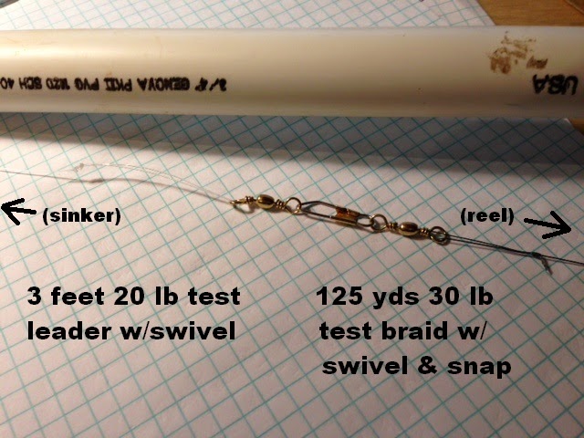
• The weight is attached to a short length of leader (about 3 feet), at the other end of which is attached a barrel-swivel.
• The main line (attached to the reel) has a barrel-swivel with snap at the end to which the leader will attach.
• Prior to making a shot, the leader's barrel-swivel is clipped to the line's snap.
• Then, after the shot has been made but before reeling a line back, simply unsnap and remove the weight and leader.  No untying knots!!!

Here's an image of the swivels and snap:

Note:  For the sinker's leader I first used some light weight mono-filament line that came with the inexpensive reel I'd purchased.  My thinking:  because I was using 30 lb. test line for my main line, if my sinker did get stuck in a tree, I wanted something that, if I pulled on it hard, would break before the 30 lb. line broke.

Unfortunately, this unknown line I used as my leader was just a bit too light weight.  On my second test shot, it parted and the sinker went sailing over the tree and out of sight.

The red arrow points to where the leader's new end.

Lesson learned.  Now I'm using 3' leaders (purchased at Walmart) that are 20 lb. test and have a barrel-swivel at one end and a barrel-swivel-with-snap at the other end.  I remove the swivel-with-snap from its end of the leader -- it's on this end that I'll attach the egg sinker.  (I can then attach one of these swivel-with-snaps to the end of my main line).  Also -- the 3 foot leaders I used come with loops in the line at their 1 foot and 2 foot marks (for attaching other hooks, I suppose).  I clip the loops open to prevent them from snagging on branch stubs, etc.

Here's a photo of the leader.  If you look closely you can see the two loops before I clipped t hem:

(click on image to enlarge)

Note regarding the leaders:  after about two dozen shots into trees, my leader (see the photo above) separated at one of the pre-installed loops -- I'm guessing that the knot used to make a loop weakened the mono-filament and it eventually parted.  For this reason, if I build more 2 oz weight leader assemblies, I'll probably just use 3 feet of the 30 lb Spider braid (that I use on my reel) in lieu of the mono-filament.

For better visibility, I spray painted the weights fluorescent orange:

Hot chile peppers in the blistering sun...

(with apologies to Dylan)

If I'm unsatisfied with the shot and decide to reel back the line for another go, I first unsnap and remove the leader and its weight and then I attach a short length of Flagging-Tape to the snap (this could be a short length of rope or string, too -- just something to add some weight to the end of the line).  This acts as a bit of drag on the end and  helps keep the snap-end of the line from flopping around and possibly wrapping around something as I'm reeling it back in.  (That's my theory, at least.)

Other notes:

• Always close the snap before reeling the line back!
• The grey 3/4" barrel was cut down from its length of 3 feet to about 30 inches so that, when the sinker has dropped down inside the barrel all the way to the barrel's bottom (make sure the valve is closed, or you'll drop through to the air chamber!), the swivel on the leader is just outside the barrel, not in the barrel.
• Useful knots:  Double-surgeon's loop knot (great for attaching swivels or making slip-knots), and the uni-uni knot (for splicing line together, which I discovered I needed to do when my more-than-200-feet of line on the reel (which I thought would be adequate) came up short in one of my shots over a very tall tree.  I'm now using the entire 125 yards of the purchased Spiderwire.) 

Final results...I can easily clear the tree in the picture below...

But how high can I get it?  The tree in the photo below is significantly higher than the one in the photo above. With 50 psi of pressure, maximum height that I can achieve seems to be on the order of 90 - 100 feet, per this photo (after shooting the weight over the branches, I reeled up the flagging-tape "tail" until it seemed about at its max height).  Note that the measurement below doesn't take into account perspective, so actual height could easily be over 100 feet:

(click on image to enlarge)

Much better than my tennis-ball antenna launcher, but can height be improved?  I'm hopeful, but nothing I've tried has yet made a significant difference. 


Standard Caveats:

Use at your own risk.  If you build one of these, don't overstress the PVC by pumping in too much air (I usually pump it up to about 40-50 psi).  Also, follow the instructions with the PVC glue, and, after handling the lead sinker and split shot, I'd recommend washing your hands.

Plus, when the weight descends, it has a lot of energy.  It has buried itself a good half-inch into the back lawn here -- I almost thought I'd lost it, then ran into the fishing line leading down into a hole in the ground.  So when you're aiming, pay attention to where it could fall!

All of which is to say: use common sense!

And, as always, I might have made a mistake in my equations, assumptions, drawings, or interpretations.  If you see anything you believe to be in error or if anything is confusing, please feel free to contact me or comment below.

And so I should add -- this design and any associated information is distributed in the hope that it will be useful, but WITHOUT ANY WARRANTY; without even the implied warranty of MERCHANTABILITY or FITNESS FOR A PARTICULAR PURPOSE.

A Milliwatt to Kilowatt RF Power Meter using the Analog Devices AD8307

A friend of mine, Dick Benson, W1QG, built a pretty cool combined Forward and Reflected Power and SWR meter using two AD8307 Logarithmic Amplifier chips from Analog Devices.  He used a PIC to convert the dBm readings back into watts (and to calibrate the device, too).

N2PK also has an interesting design for a "Forward Power and Return Loss Meter."  It, too, uses two AD8307 ICs.

One of these days I'll build a "Power and SWR" meter, too, but for the lab bench I thought a basic Power Meter would suffice.  Almost all of my work on transmitters is either testing or repairing them, so I don't really need to measure SWR or Reflected Power.  With that thought in mind, why not design a 0 - 60 dBm (1 milliwatt to 1000 watt) power meter?

Here's a picture of the completed power meter.  It reads either 0-30 dBm (1 - 1000 milliwatts) or 0-30 dBW (1 - 1000 watts).  Yes, the scale is in milliamperes.  Someday I'll make an appropriate scale.  But meanwhile, it's easy enough to convert the 0-3 mA scale to 0-30 dBm/dBW.

(click on image to enlarge)

And here's the schematic:

(click on image to enlarge)

And here's a better version, drawn after I'd posted the one above...

(click on image to enlarge)

Choice of parts (apart from the AD8307) was pretty much dictated by what I had in my junkbox.  The case was originally from a Drake W4 wattmeter. (I no longer recall where I found the case -- I must have picked it up (sans meter and electronics) at a swapmeet sometime in the past).

The meter (0-3 mA) was chosen because it was in the junkbox and, most importantly, it fit the hole in the case's front panel!  I initially wanted to use a meter that was marked from 0 to 600 mA (actually a 100uA FS meter), because the scale would be perfect for a 0-60 dBm meter without a range switch.  But I really wanted to avoid cutting a meter hole, so the 0-3mA meter won out.  The 0-60 dBm overall range is now broken into two sub-ranges:  0-30 dBm and 0-30 dBW (i.e. 30-60 dBm).

I also wanted to used op-amps with rail-to-rail outputs (so that I could drive down to 0 volts).  Fortunately, I happened to have some TLC2272 op amps on hand.


Schematic Notes: 

The design uses 5VDC, provided by a 78L05 regulator that drops the input DC (e.g. 9V - 20V) down to 5V.  The 1N4148 is just there to provide circuit protection in case the wrong polarity DC is attached to the input.

The AD8307 has a 92 dB Dynamic Range (-75 to +17 dBm), but if you look at the charts in the datasheet you'll see that accuracy suffers a bit at the ends of this range -- I think a range from -60 to +10 dBm is more reasonable if you want to preserve accuracy.  So I decided to limit my top-end to +10 dBm, which would put my bottom end at -50 dBm.

50 dB of attenuation (externally applied) is required to drop the "application" power range of 0 - 60 dBm down to the meter's input range of -50 to +10 dBm.  Not a problem, as I'll explain later.

The 52.3 ohm resistor to ground at the BNC input parallels the AD8307 input impedance (1.1K || ~0.7pf) and brings it closer to 50 ohms.  (Note, the 0.7pF would be the differential input capacitance.  I.e. 1.4 pf to ground (for each input pin), in series).  Here's an S11 plot of the Input port's Return Loss:

Because of the lower power levels that the AD8307 would be working with, I decided to shield the AD8307 to (hopefully) prevent external RF fields from affecting the reading.  I built the sides of a small shielded box on the ground plane using copper-clad PC stock. Copper tape (soldered to the box sides) caps the box.

Power and the output signal from the AD8307 pass through the box via feedthrough caps (1nF, if I recall their value correctly).

I amplify the AD8307's output signal, whose slope is about 25mv/dB, by a gain of 4, which increases the signal's slope to 0.1V/dB (i.e. 1V/10dB).

For the op amp to generate 0-3V for each of the two ranges, given that the AD8307 output ranges from about 0.9V to 2.4V over an input range of -50 to +10 dBm, I have two switchable "offsets" that connect to the negative-input of the op-amp, thus shifting the AD8307's output down so that 0 dBm (or dBW) corresponds to 0V out of the op amp and a reading of 30 (dBm or dBW) corresponds to 3V.

A "Range" switch (0-30dBm or 0-30 dBW) selects a "course" DC offset, which then can be fine-tuned with the "ZERO" pot.  The pot spans the same amount of voltage, but shifted, when the range switch is toggled (because the total resistance in the voltage divider does not change).  Note that changing ranges requires re-zeroing the meter. 

Two more op amps round out the design.  The first drives a 10 uF cap, which acts as a peak-hold (with its "slow" decay determined by a parallel 1 Meg ohm resistor. This feature is useful when looking at peak-power.  The op amp drives a 2N3904 transistor which is in the feedback loop.  This transistor serves two purposes -- it provides adequate current to charge up the 10 uF cap (the TLC2272 is a bit wimpy), and its base-emitter junction blocks the cap from discharging through the op amp when the output of the op amp drops down below the capacitor's voltage.

Note that the 2N3904's V_(BR)EBO is 6V (min), which is greater than the 5V powering the TLC2272 driving the 2N3904's base.  So there's no danger to the transistor's Base-Emitter junction when the 10uF cap's voltage is high and the op amp's output is low.  By the way, I used 2N3904 transistors because I have a bunch on hand.  2N2222  transistors or any other garden-variety NPN would be fine, just as long as it has a minimum Beta of at least, say, 20, and a V_(BR)EBO of at least 5V.

A switch allows selection of "slow" or "fast" decay of the peak-hold cap by switching in a 10K resistor to parallel the 1 Meg "slow" decay.

The other op amp drives the meter and isolates the peak-hold cap from the relatively low resistance represented by the meter.  The 500-ohm pot acts as a "Gain" control and it ensures that the reading of the analog front-panel meter correctly corresponds with the input power.  Initial setup requires a bit of tweaking between this control and the "Zero" control to get the meter's needle to read correctly from 0 to full-scale, but once it's calibrated, one shouldn't need to touch the "Gain" control again (thus, it's on the back panel).

A second 2N3904, in the feedback loop of this meter-drive op amp, provides current gain for the its TLC2272.  These op amps are a bit anemic with respect to current-drive, and their output voltage can drop appreciably with loading.  The transistor's current amplification keeps my 3 mA meter from loading down the op amp's output.

If better accuracy is desired, I can read power via an external DVM rather than use the front-panel's analog meter.  A separate BNC connects a DVM to the output of the meter-drive op amp output -- remember, this output goes from 0 to 3V with a slope of 1V/10dB.  There's a series 10K just to limit current in case ESD somehow hits this signal, but it has no effect on the DVM reading, due to the DVM's much higher input impedance.

Additional thoughts:

I used TLC2272 op amps because that's what I had on hand, but these devices cannot source much current (e.g. the 3 mA required for my meter) without experiencing significant voltage drop at their outputs.  A better choice would be the LMC662 family used by N2PK in his Power Meter.  This device would allow you to eliminate both 2N3904 transistors, with the 2N3904 used for the peak detector replaced with a simple diode, e.g. 1N4148.

Something else to try would be to replace the single "Zero" pot with two pots, each selected by the Range switch.  I'd tried to select my voltage divider so that the single pot wouldn't need much tweaking (ideally: none) when flipping between the range switch, but I wasn't successful.  If it turns out that the zero pot, over time, needs no retweaking for a given range, then there's no reason why the single pot couldn't be replaced with two pots mounted, say, on the back panel, instead of on the front panel.

Notes on Construction:

I like to build on copper-clad PC stock because it provides a great ground plane for the circuitry (and I have quite a bit of it in my junk box).  When mounting IC's, I'll mount them "top-up" so that I can see their part numbers.  Pins going to ground are bent down and soldered to the copper plane.  All other pins are bent out so that they are straight out from the sides of the IC (like the wings of an airplane).

To give the device stability (in case, say, only one pin goes to ground), I'll solder a power-bypass cap to the board so that it's lying on its side and then solder the IC power pin to the other lead of the cap.  Or I'll solder a high-value resistor (e.g. 1 Meg) to the board next to a pin.  The resistor sticks up straight and will support the side of an IC that has a pin soldered to to the top of the resistor.

Here's the start of the build...

(click on image to enlarge)

Bending pins is great if you're using DIP packages, but often I'll be using SOIC parts.  What I try to do for these is to purchase little prototyping boards designed to adapt specific SOIC packages (e.g. SOIC-8) to DIP spacing.  I'll then stand these proto boards off the copper plane using either leaded 1 Meg resistors or, where appropriate (e.g. Ground), stiff wire.

In the picture below the two small green boards are the prototyping boards for the two TLC2272 packages.  (You can often find these on eBay).

And here' the completed unit!

To make the front panel overlay I used the same technique that I describe here.


In Operation:

In the photo below the meter is reading 10 dBW (i.e. 40 dBm, or 10 watts), and the DVM is connected to the meter's "To DVM" port, whose output slope is 1V per 10 dB (thus the 1V reading for a 10 dBW signal).

By the way, in the photo above I'm not really driving the meter with a 40 dBm signal -- if no external attenuation is used, the meter's "0-3 mA" scale can be spanned by an input signal ranging from -20 to +10 dBm (when the "Range" switch is in its "High" position (30 dBW)).  Only with an external 50 dB attenuator will the scale accurately reflect the actual power (e.g. 0-30 dBW or 0-30 dBm).  So, in the photo above I'm actually using no attenuation and I'm driving the meter with a -10 dBm signal from my RF Generator.

So it's worthwhile noting that other values of attenuation can be used in lieu of 50 dB.  The table below shows how the measurement range would shift with different values of input attenuation.  For example, if I used 20 dB of external attenuation and set the Range switch to its Low (30 dBm) position, then I could directly measure (using the meter's scale) 0-30 dBu (dB microwatt).

External 50 dBm Attenuator:

As I mentioned earlier, this design requires some form of external attenuation for the 0-60 dBm measurement range.  Fortunately, the shack/lab here has a variety of ways to attenuate RF signals:



(Back:  Bird 200 watt, 30 dB attenuator.  Front-left: 50 watt dummy load with 50 dB attenuator.  Front-right: homebrew -24 dB directional coupler.)

When testing and repairing transmitters, I usually use this setup:

Although the dummy load (military DA-437/GRC-103(V)) is rated at 50 watts, it seems to work fine with 100 watt transmitters (admittedly I minimize "key-down" time).  The 40 dB attenuator is just a voltage divider that divides the voltage at the dummy load (e.g. 70.7 volts @ 100 watts) by a factor of 100 (40 dB).  I chose this scheme of attenuation because it doesn't require the attenuator to dissipate large amounts of power and the 2.5K ohms has little impact on the 50 ohm impedance seen by the transmitter.

Here's what the 40 dB attenuator looks like:

(click on image to enlarge)

The series 2.5K resistor was tweaked (by paralleling another resistor) to give 40 dB +/- 0.15 dB of attenuation (while attached to the dummy load) over the range of 1 to 54 MHz.  (To keep the frequency response flat over that range I had to add a capacitive "gimmick" to ground next to the series resistors -- essentially some copper tape tied to ground that I wrapped around the resistor bodies). 

Note, too, that if driving the dummy load with 100 watts of power, the 2.5K resistor will need to dissipate about 2 watts, so select values accordingly. And to get 40 dB of attenuation there needs to be a 50 ohm load (e.g. the input of a spectrum analyzer) connected to the output (attenuated) port. 


Converting dBm to Watts:

To convert dBm to Watts, you can use the formula:

Power(watts) = (0.001)*10^(dBm/10) 

But the table below might be simpler to use:

These readings can be easily scaled to other powers.  For a given dB range, multiply the milliwatt reading by the appropriate power of 10.  For example:

• For the range 0-10 dBm, multiply "milliwatts" by 1
• For the range 10-20 dBm, multiply "milliwatts" by 10
• For the range 20-30 dBm, multiply "milliwatts" by 100

So, if a reading is 11 dBm, the power would be 13 milliwatts.  Similarly, 21 dBm would be 130 milliwatts.

If the Range switch is set to 30 dBW, then "milliwatts" is replace by "watts", and a meter reading of, say, 11 dBW would correspond to 13 watts.


References:

N2PK Forward Power and Return Loss Meter  Design using two AD8307 Logarithmic Amplifiers.

Analog Devices AD8307 92 dB Logarithmic Amplifier, Datasheet

TI TLC2272 Dual Rail-to-Rail Op Amp, Datasheet


Links to my Directional Coupler blog posts:

Notes on the Bruene Coupler, Part 2

Notes on the Bruene Coupler, Part 1

Notes on HF Directional Couplers

Building an HF Directional Coupler

Notes on the Bird Wattmeter

Notes on the Monimatch


Standard Caveat:

As always, I might have made a mistake in my equations, assumptions, drawings, or interpretations.  If you see anything you believe to be in error or if anything is confusing, please feel free to contact me or comment below.

And so I should add -- this design and any associated information is distributed in the hope that it will be useful, but WITHOUT ANY WARRANTY; without even the implied warranty of MERCHANTABILITY or FITNESS FOR A PARTICULAR PURPOSE.

More Notes on Directional Couplers for HF -- the Bruene Coupler, Part 2

This is Part 2 of my notes on the Bruene Directional Coupler.  Part 1 is >>here<<.  I strongly suggest reading Part 1 -- it explains a more easily understood variation of Bruene's circuit.

So, assuming you're familiar with the basic principles of the Bruene coupler, let's move on to Bruene's design!

Let's start with the schematic of the Bruene Coupler:

(click on image to enlarge)

This coupler was used in the Collins 302C-3 Directional Wattmeter and it was also described in an article written by Warren Bruene in QST magazine ("An Inside Picture of Directional Wattmeters," QST, April, 1959).

This architecture uses the same principles as the ones described in Part 1:  to generate a voltage representative of a Forward Wave on a transmission line, a sample of the line current is added to a sample of the line voltage.

And to generate a voltage representative of a Reflected (or Reverse) wave on a transmission line, a sample of the line current is subtracted from a sample of the line voltage.

What differentiates Bruene's design from the other variations is that those variations keep the circuitry generating the voltage sample independent of the circuitry generating the current sample.  Which is to say, with those other designs I could take a voltmeter and independently measure the voltage sample and the current sample.  I cannot do that with Bruene's circuit -- voltage-sample and current-sample generation are bound together!

You're probably looking at the above schematic right now and wondering what the heck I'm talking about.  You see two voltage dividers, so they must be generating the voltage sample of the Transmission Line voltage, while the transformer (with the two 10 ohms resistors) is generating a positive and negative voltage related to the current on the Transmission Line.  Everything's copacetic, right?

But take a closer look.

Vfwd and Vref. which are the sum and differences of the voltage and current samples, are measured at the divider-taps of the two capacitive voltage dividers.  So the voltage dividers can't just be generating samples of the Transmission Line's voltage.  They must somehow be involved with summing in the Line current samples, too!

The key to the summing are the two diodes. But how are the diodes doing this?

Each diode is actually behaving as a "shunt rectifier" (see Chapter 2 in this >reference<).  And this shunt-rectification process is differencing (rather than summing) the voltage-sample and the current sample that are at the diode's Cathode and Anode, respectively, with the result appearing at the diode's Cathode (the junction of the two voltage-dividing capacitors).

To illustrate this concept better, I've done some basic simulations using LTSpice.  My simulation-circuit is a much simplified version of the part of Bruene's coupler that generates Vref.  Please note that:

1. I use the same capacitor values for the voltage divider as Bruene.  Vsource is the voltage across the transmission line.  It's a large amplitude because the voltage divider has a huge division ratio.
2. The voltage created by the current-sampler, originally generated by a current source (the transformer) driving its current through the resistors, has been replaced by its Thevenin equivalent, but I've made the series-R very small to keep its effect from confusing this discussion.  I've called this voltage source Vinduced.
3. I've added a "switch" between the Diode's anode and Vinduced so that I can look at the voltage sample (at the voltage-divider tap) for a full 360 degree cycle without it being influenced by the current sample.

Below is my first simulation.  To illustrate the shunt-diode's operation, we will first simulate Vinduced as a DC voltage source of 0 volts.  For the shunt-diode I've chosen a 1N916 (a silicon diode).  The actual circuit uses Germanium diodes (I believe).

I've annotated the schematic below to describe the basic functions of each part of the simulation circuit.

(click on image to enlarge)

So what's going on in the plots?  Let's look...

(click to enlarge)

I've defined an "Offset" voltage across C2.  It can also be thought to be across C1, too, and it's effectively the amount that Vsample has been shifted.  I'll explain this further a bit further down the post.

Looking at the plots, at 100nS we connect Vinduced to the diode and so at the 150 ns mark, when the voltage at Vsample is driven negative by Vsource, the diode's cathode connected to Vsample will start to go negative during the negative half-cycle of Vsource.  Because the diode's anode is tied to a 0V source, the diode will turn ON when its cathode voltage drops about 0.7V below its anode voltage.  I.e. when Vsample is approximately -0.7V.

When the diode turns ON, it effectively "clamps" the voltage at Vsample to -0.7 volts.

However, Vsource is still going negative.  So we have the "+" terminal of C2 (see simulation schematic) clamped at -0.7V and C2's "-" terminal (attached to Vsource) continuing down, which causes charge to flow onto C2's plates.   When Vsource reaches its negative peak, this charge can be calculated from the equation Q = C*V:

Q(max) = C2*Vsource(pk)

Actually, in the real world the voltage is slightly less than this by Vf, the forward voltage  drop across the diode.

Now, as Vsource starts to rise again from its negative most transition, the diode turns off, but not immediately, which is the "real-world" diode turn-off effect you see on the Red line in the plot above.

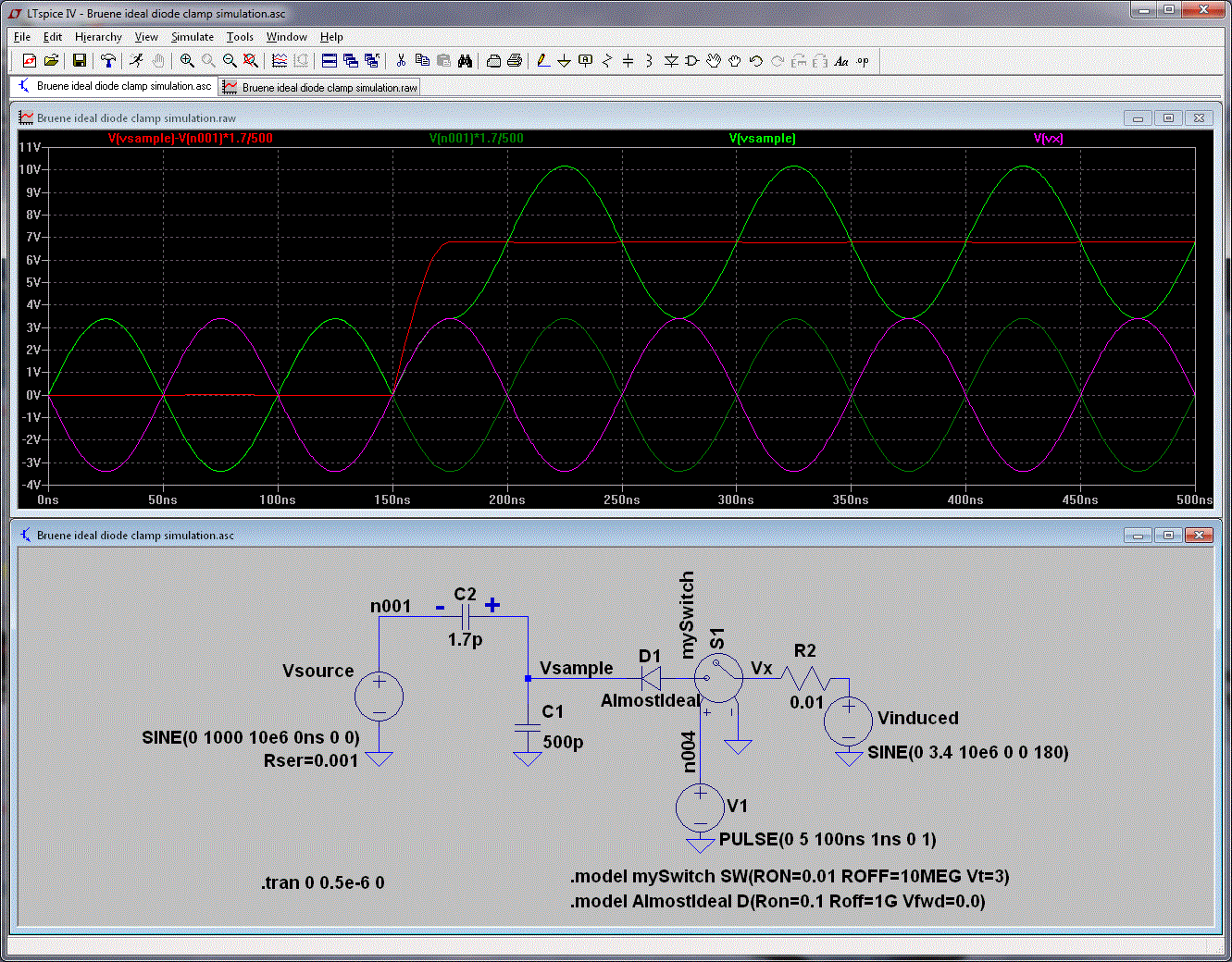
With real-world diode effects, the plots can get a bit confusing, so let me introduce a simpler example that uses an "ideal" diode.  I'll define the diode to have a Vf of 0V:  if its Cathode is at all negative with respect to its Anode, it is ON, and if its Cathode is at all positive with respect to its Anode, it is OFF.

Shunt Rectifier with Vinduced as a DC source and an Ideal Diode:

Here's the circuit and the simulation:

 (click on image to enlarge)

 

Looks a bit cleaner, doesn't it?

So what is happening?

From 0-100ns the diode's Anode is floating because the switch is open, and it is essentially out of the circuit.  Vsample is just Vsource divided down by the capacitive voltage divider (C1 and C2), and therefore Vsample goes between -3.4V and +3.4V.  Its average value is 0V.

At 100ns the switch turns ON, and the diode's Anode is connected to Vinduced, which here is a 0VDC source.

From 100ns to 150ns, Vsource is positive and thus Vsample is still positive.  The diode is OFF (it is back-biased:  Cathode positive, Anode at 0VDC), and Vsample is still just Vsource divided down by the capacitive voltage divider (C1 and C2).

But starting at 150ns, Vsource goes negative and it tries to take Vsample below 0, too.  But Vsample cannot go negative, because as soon as it begins to go below 0V, the diode turns ON and clamps it to the voltage at its Anode, 0VDC.

So as Vsource goes negative, Vsample sticks at 0V, and the voltage across C2 (1.7pf) gets larger and larger, until, at 175ns when Vsource is at its negative peak, the voltage across C2 (Vc2) is at its max:

Vc2(max) = 1000 V.

At this point C2 will have its maximum charge on its plates.  From the formula Q = C*V, we know that:

Qc2 @ max V = C2 * Vc2(max) = C2*Vsource(peak)

(...given the voltage at the diode's Anode is 0VDC and that the diode is ideal with a 0V Forward-voltage drop.)

Also, note that the voltage across C1 (500pf) is 0V (Vsample is clamped to 0V).  Therefore the charge on C1 is 0 coulombs.

So at 175ns, when Vsource has reached its most negative excursion, the maximum charge is on the two caps:

Qmax = Qc1 + Qc2 = 0 + C2*Vsource(peak)    (equation 1)

Now, as time moves on from 175ns, Vsource just starts to rise up from its negative peak. Vsample, which was at 0 V, starts to go positive and the diode immediately cuts off (because Vsample = Vsource + Vc2(max)).  The diode is now effectively out of the circuit.

The diode is back-biased and out of the circuit.  There's no path for the charge of Qmax on C2 to go but to C1 (there's no other path but to C1).  So, as time continues, no charge will by lost by the C1/C2 combo, and no charge will be added -- the diode never turns on again.  And so the total charge on C2 and C1 (=Qmax) will flow back and forth between C2 and C1 as Vsource goes up and down.

No charge is being added, no charge subtracted.  Therefore, at all times (after we've first charged C2 via the diode clamp), the charge across C1 and C2 must satisfy this equation:

Qc1 + Qc2 = Qmax

And therefore (using Q = C*V):

C2*(Vsample - Vsource) + C1*Vsample = Qmax

Rearranging:

Vsample = Vsource*C2/(C1+C2) + Qmax/(C1+C2)   (equation 2)

So, if we know Qmax (and we do), we can calculate what Vsample will be for any value of Vsource.

The equations above do this for an ideal diode with 0V attached to its anode.  We can derive a more general equation for Qmax (rather than use equation 1 above) that takes into account the voltage connected to the diode's Anode and also its Forward-voltage drop (i.e. a non-ideal diode):

Qmax = C2*(Vsource(pk) + V(anode) - Vf(diode)) + C1*(V(anode) - Vf(diode))   (equation 3)

Using equations 2 and 3, we can now calculate Vsample for different voltages connected to the diode's Anode, per the table below (I'll keep the diode ideal, though, with Vf = 0):

(click on image to enlarge)

You can see that "Vsample without diode" ranges from -3.4 to 3.4V.  If we look at, say, the diode with 0V attached to its anode, the range of Vsample now becomes: 0V to 6.8V -- a shift of 3.4V, the peak voltage of the non-diode Vsample.  So Vsample's average voltage is now 3.4 volts instead of 0, and if we were to filter out the AC waveform on Vsample we would measure 3.4 VDC.

The previous example was with a DC source connected to the diode's Anode and demonstrates how the shunt-rectifier can create a DC voltage from an AC signal.  What happens if the Anode is instead connected to an AC source representing the voltage from the current-sample?


Vinduced as an AC source:

So all is fine and good if Vinduced is a DC source.  Let's change Vinduced from a DC voltage source to something instead the simulates what is actually happening in the Bruene Coupler -- an AC source of the same frequency as Vsource, but with a phase offset.

We should still see a DC offset voltage generated on the capacitors in an analogous way to when Vinduced was a DC source. But the level of this offset voltage should now depend on the phase difference between the Vinduced and Vsource.

To keep the analysis simple, I won't be changing the amplitudes of Vsource or Vinduced, just their phase relationship.  And note that the amplitude of Vsource has been chosen so that, if the diode were removed, Vsample = Vinduced in amplitude.  

Let's examine how the voltage offset changes with phase (see the RED line in the plots below).  With the two waveforms 180 degrees out of phase, LTSpice simulates this value to be 6.8V:

(click on image to enlarge)

With the two waveforms 180 degrees in phase (0 degrees delta), LTSpice simulates this value to be 0V:

(click on image to enlarge)

 

With the two waveforms 45 degrees out of phase, LTSpice simulates this value to be 2.61V:

(click on image to enlarge)

With the two waveforms 180 degrees out of phase, LTSpice simulates this value to be 4.8V:

(click on image to enlarge)

 

And finally, with  the two waveforms 135 degrees out of phase, LTSpice simulates this value to be  6.28V:

(click on image to enlarge)

Summarizing the DC offset calculated by the simulations:

But is this DC value that LTSpice calculates actually equal to the difference (or sum) of the two sine waves representing our voltage sample and current sample?  This is a requirement that must be met if we are to calculate Vfwd and Vref by adding or subtracting the voltage and current samples.

Let's check this by doing some separate math, using the same peak voltages and phases that I used in the LTSpice examples above...

If summing sine waves, I can use the following equations to calculate the the resulting amplitude of the summed waveform (amplitude can be expressed as Vrms, Vpp, etc.  I'll use Vpeak, which, from our simulations, is 3.4V).

Knowing the amplitudes of the sine waves and the different phases, I can plug these numbers into Excel and solve for c, the summed-amplitude (called Vc in the table, below):

(click on image to enlarge)

The "LTSpice" column is 180 degrees out of phase with with "formula" column because the "shunt-diode" circuit is actually a differencer, not a summer, which is equivalent to adding 180 degrees to the phase shift "α" in the formula for c.

If we compare the table results from the math with our simulation results (see the earlier table), we find that they are exactly the same values (after first taking into account the shunt-diode's additional 180 degree phase shift).  Which means that the shunt diode circuit is indeed summing (or differencing) the voltage waveforms of the voltage sample and the current sample!

And therefore, it is functionally equivalent to the earlier Bruene coupler variants that we looked at in Part 1.

Now that I've shown that the shunt-rectifier sums or differences the voltage and current samples, I'll refer you back to Part 1 for a recap of circuit operation in Transmission Line and non-Transmission Line environments.

The only thing to keep in mind is that, because the shunt-rectifier is actually a differencing circuit, not an adder, the side of the coupler that, in part 1, generated Vfwd (that is, the left side of the circuit in the diagrams), now generates Vref.

And the opposite side (the right side of the circuit in the diagrams) now generates Vfwd.

Other than that, the same analysis applies!


Bruene Variant, Daiwa SWR Meters:

While looking around the shack I came across a Daiwa CN-620B wattmeter that I pickup up several years ago.  Opening it up, I discovered it's a variation of the Bruene Coupler that uses Bruene's "shunt rectifier" method of creating a DC voltage from the voltage and current samples.

(click on image to enlarge)

Inside the Daiwa CN-620B (click on image to enlarge))

 The main differences that I can see between it and Bruene's design are:

• Daiwa uses two transformers, one for Vref for Vfwd, compared to Bruene's one.
• The Daiwa transformers have fewer windings than Bruene's (I believe the latter has 60).

A number of other Daiwa wattmeters (e.g. CN710, CN720) use the same or similar design.  Curiously, when I look at the values of the components on the CN-620B's PCB, they are significantly different than the values listed in the schematic! Don't know why.


Links to my Directional Coupler blog posts:

Notes on the Bruene Coupler, Part 2

Notes on the Bruene Coupler, Part 1

Notes on HF Directional Couplers (Tandem Match)

Building an HF Directional Coupler

Notes on the Bird Wattmeter

Notes on the Monimatch

Notes on the Twin-lead "Twin-Lamp" SWR Indicator

Calculating Flux Density in Tandem-Match Transformers


And some related links from my Auto-Tuner and my HF PA posts:

Auto Tuner, Part 5:  Directional Coupler Design

Auto Tuner, Part 6:  Notes on Match Detection

Auto Tuner, Part 8:  The Build, Phase 2 (Integration of Match Detection)

HF PA, Part 5: T/R Switching and Output Directional Coupler


Bruene Coupler References:

Bruene, Warren, "An Inside Picture of Directional Wattmeters," QST,  Apr., 1959.  Includes both a good explanation of the Monimatch operation and a design for a directional wattmeter whose directional coupler topology would later be known as the "Bruene Coupler."

Collins 302C-3 Directional Wattmeter, PDF Manual containing schematic.

Rush, James, Jr., "The Mini-Mono-Monimatch," QST, Mar., 1965.  Although called a Monimatch in the title, the design is actually more similar to Bruene's directional coupler.

Bold, Gary, ZL1AN, "The Bruene Directional Coupler and Transmission Lines," PDF. This PDF gives an excellent explanation of the Bruene Coupler.

Kiciak, Paul, N2PK, "An HF In-Line Return Loss and Power Meter," PDF.  Constructions details of a power meter using a Bruene Coupler.  Contains an explanation by the other of why he prefers the Bruene coupler of the Tandem-Match Coupler.  Also interesting because the author separates the voltage-sampler from the current sampler and uses the differential inputs of an AD8307 to do the required addition (or subtraction) to get FWD and REF voltages.

(This web page could be useful for understanding the sampling method used in the N2PK meter:  http://www.g3ynh.info/zdocs/bridges/magdiff/part1.html )

Lewallen, Roy, W7EL, "A Simple and Accurate QRP Directional Wattmeter," QST, Feb, 1990, PDF.  Interesting variant of the Bruene coupler.  Roy uses two transformers for the voltage sample in lieu of capacitor voltage dividers.

White, Ian, G3SEK, "Inside a Directional Wattmeter," RadCom, Sept., 2002, PDF.  Discussion and a bit of analysis of Bruene coupler.  Includes Bruene's phase-relationship diagrams.

http://www.g3ynh.info/zdocs/bridges/reflectom/part1.html  interesting analysis

http://www.g3ynh.info/circuits/Diode_det.pdf  Diode detectors -- includes some info on shunt detectors, which is what Bruene's design uses.


Other references of generally interest:

http://www.g3ynh.info/zdocs/bridges/Xformers/part_1.html  great discussion on current-transformers for directional coupler applications

http://www.g3ynh.info/zdocs/bridges/Xformers/part_2.html Part 2 of current-transformers

http://www.g3ynh.info/zdocs/bridges/Xformers/part_3.html  And part 3, the last part, of current-transformers

http://www.g3ynh.info/zdocs/bridges/index.html  Indexes numerous topics.  Lots of great info to be found here!

http://www.richtek.com/assets/AppNote/AN008_EN/AN008_EN.jsp  Common-Mode choke model


Final Caveats:

As always, I might have made a mistake in my equations, assumptions, or interpretations.  If you see anything you believe to be in error, or if anything is confusing, please feel free to contact me.