(Update, 10 November 16. Added W3MQW's Tuning Detector from the
November/December, 2016 issue of QEX. See item 7, below.
Also, many of my comments below (regarding W3MQW's Tuning Detector) are
published in my "Letter to the Editor," in the March/April 2017 issue of
QEX.)
This is the sixth blog post in my Automatic Antenna Tuner Series.
(The fifth post, dealing with Directional Coupler design, is
here).
Why match detection?
It seems to me that many microprocessor-based tuners use an SWR-based approach
to tuning. That is, they step through their components, looking for a
trend in which the SWR decreases. Once a trend is found, the
tuning-algorithm can refine its tuning step size and (hopefully) locate an SWR
minima.
With an L-network tuner there should only be one SWR minima (unlike a
T-network tuner). So, as long as the load SWR is within the tuner's
matching range, and as long as the component step sizes are small enough, the
algorithm should be able to tune the SWR down to meet the designed-for goals
(e.g. SWR less than 1.5:1).
But I've never been impressed by this method of tuning. Should an
L-Network tuner start in the LsCp configuration or in the CpLs
configuration? It's a toss-up.
And the tuning-algorithm must hunt around, searching for a declining SWR
trend, before it can continue to tune to a minimum SWR.
So, there are two reasons to be dissatisfied with an SWR-only algorithm.
But do better ways exist? Could it be that SWR-tuning is the best
choice?
So, as part of my design effort, I thought I'd explore other
Match-Detection/Tuning methods.
Other Match-Detection Methods:
In addition to measuring SWR, here are some other parameters that can be
measured.
-
Detect phase of transmission-line current versus voltage. Tune for
zero phase difference.
-
Detect the magnitude of the load's impedance (|Zload|) and tune it to be
equal to 50 ohms.
-
Detect the value of the load's Resistance (Rload) and tune for it to be
equal to 50 ohms.
-
Detect the value of the load's Conductance (Gload) and tune it to be equal
to 20 millimhos.
Non-SWR tuning schemes seem to apply phase-detection in combination with one
or more of the other three measurements above.
Let's look at some applications of these match-detection methods:
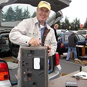
1. Tuning Detector, AN/GRC-106
The AN/GRC-106 (and AN/GRC-106A) is a military HF transceiver first introduced
in the 1960's.
Although it doesn't have an automatic tuner, it has two "tuning" meters (ANT.
TUNE and ANT. LOAD), and the detection circuitry that drives these two meters
is similar in function to the match-detect circuitry in other radios. So
this radio provides a good starting point for understanding a couple of basic
tune-detection blocks.
(Photographed at the De Anza Swapmeet, 07/15)
Let's start with the schematic of the GRC-106's tuning detectors. There
are two functional blocks. One block detects the phase difference
between transmission-line voltage and transmission-line current (the GRC-106
documentation calls this block the "Tune Discriminator").
The second functional block detects if the magnitude of the load impedance is
more or less than 50 ohms. (This block is name the "Load
Discriminator").
Both functional blocks are shown in the schematic below.
(click on image to enlarge)
The GRC-106's
Tune Discriminator has a single function -- to indicate
to the operator when the transmission-line current is
in-phase with the transmission-line voltage. An
in-phase
condition means that, to the radio, the load appears to be solely resistive,
without any reactance.
On the other hand, the
Load Discriminator indicates to the operator
when the load has been tuned to look like a 50 ohm
impedance. Note my stress on the word
impedance -- this detector
simply indicates if the
magnitude of the load's impedance looks
like 50 ohms -- it has no idea if the 50 ohms is resistive, reactive, or a
combination of the two.
So -- if the Tune Discriminator indicates 0 phase and the Load Discriminator
indicates 50 ohms, then the antenna has been tuned to look like 50 ohms,
resistive. The operator will have tuned the radio's network to a 1:1
SWR!
Let's now look more closely at these two circuits...
The GRC-106 Tune Discriminator:
When a load is purely resistive, the transmission-line voltage is in-phase
with the transmission-line current (i.e. 0 degrees phase delta between the
two).
But if the load is inductive, the transmission-line current will lag the
transmission-line voltage. And if the load is capacitive, the current
will lead the voltage.
The GRC-106 Tune Discriminator detects the phase difference between
transmission-line voltage and current, generates a DC voltage proportional to
this phase difference, and applies this voltage to a "center zero" panel meter
(see the picture of the front panel, above).
(click on image to enlarge)
The secret to this circuit's operation is a 90 degree phase-shift
introduced to the current sample. That is, the voltages induced at
the secondary of the current-sense transformer are 90 degrees out of phase
with the transmission-line current passing through the transformer's
primary. So, if transmission-line voltage and current are exactly in
phase on the line, they are out of phase by 90 degrees in this circuit.
Looking into the circuit a bit further... The transmission-line
voltage is "sampled" with a capacitive voltage divider (formed by C4 and
C1 in the schematic below). If the line voltage is "v", then the
sampled-voltage is v/N.
(click on image to enlarge)
T1 can be analyzed as three coupled-inductors. One inductor is simply
the "one-turn" of wire passing through the center of the core. The other
two will have voltages induced across them that are equal to j*2pi*F*M*i,
where F is frequency, M is the Mutual Inductance, and i is the current in the
primary.
To illustrate phase-discriminator's operation, I've created a simple SPICE
example. (Please note that the 2.5mH inductor simply provides a DC path
to ground for the transformer center-tap):
(click on image to enlarge)
(I used 4 turns for each secondary for purposes of simulation and
illustration. But I don't know what the winding ratio really is.)
With a 50 ohm load (no reactance), transmission line current and voltage are
in phase. In the image below, please note the following:
-
The voltages across the two windings, L2 and L3, are equal in magnitude
and always in-phase (when referenced to their winding phase "dots").
The graph below plots these inductor voltages, Vb-Vc and Vc-Va (and
because they equal each other, you only see one trace, not two -- the
Vb-Vc traces sits on top of the Vc-Va trace).
-
The two inductor voltages are 90 degrees out of phase from the
transmission line voltage.
(click on image to enlarge)
Va is created by
adding the voltage across L3
to the
voltage-sample, Vc, and Vb is created by
subtracting the voltage across
L2
from the voltage-sample, Vc.
In this example with a resistive load, because the line current is in-phase
with the line voltage, and even though one inductor voltage is being added to
the voltage sample that is 90 degrees out of phase with it and the other
subtracted from that same out-of-phase voltage, the resultant waveforms will
still have the same magnitudes.
I've plotted these resulting voltages, Va and Vb, below. Note that,
because the load is a 50 ohm resistor (no reactance), Va and Vb are still 90
degrees out of phase from both the transmission line current and
voltage. And they are 180 degrees out of phase from each other, but
their amplitudes are equal.
(click on image to enlarge)
Now let's change the load from 50 ohms resistive to 50 + j100 ohms (series
inductance of 1.6 uH). The voltage sample's phase with respect to the
voltage generated across the inductors is no longer out of phase by 90
degrees. And so when the inductor voltages are summed-with, or
subtracted-from, the voltage sample, the resultant waveforms will have
different amplitudes.
In the case of this particular reactive load, Va is now larger than Vb.
(Note that Va and Vb are still +/-90 degrees out-of-phase from the current (as
they should be, given that the voltages across L2 and L3, by definition, are
shifted from the line current by 90 degrees).
(click on image to enlarge)
If I change the load to 50 -j100 (series capacitance of 160 pF), the
line-voltage now lags the line-current, and Vb is now larger than Va.
(click on image to enlarge)
Two important notes regarding this type of phase discriminator:
-
For the 90 degree phase-shift to exist across the transformer's
secondaries, the load across these secondaries should be high (i.e.
ideally the secondaries would be unloaded).
-
And if the load across the transformer's secondaries is high, then the
primary's inductance should be a small inductance so that it,
itself, does not add additional phase-shift to the transmission line
current.
I explain both of these points further in the
Notes on Modeling Transformers section, below.
By the way, more details on the operation of the GRC-106 phase discriminator
can be found in the
Technical Manual
(page 1-60).
And before I leave this topic, just a quick explanation regarding the math
involved...
I can describe Va and Vb in terms of Vc, the voltage-sample (from the
capacitive voltage divider), and Vi, the current-sample voltage induced across
a secondary winding:
Where 'α' represents the phase shift between the two voltages (normally 90
degrees with a resistive load).
For the purposes of illustration, I'll keep the math simple and assume Vc = Vi
= 1, which will allow me to apply the following trig identities:
Substituting 'xt' for 'u' and 'xt + α' for 'v' in the equations above, the
result is:
The magnitudes of these two voltages are:
Clearly if α is 90 degrees (i.e. resistive load), these two magnitudes are
equal (sin(45°) = cos(45°) = 0.707). But as transmission-line voltage
shifts in phase from transmission-line current, α will shift from 90 degrees
(either towards 0 degrees or towards 180 degrees), and these two magnitudes
will no longer be equal.
At the limit of α = 0 degrees, |Va| will be 2 and |Vb| will be 0. And at
the other limit of 180 degrees, |Va| will be 0 and |Vb| will be 2.
(And please note: you can also find the operation of this type of
phase-discriminator described in terms of Phasors, below, in the Collins
180L-2 section).
The GRC-106 Load Discriminator:
The load-discriminator's operation is straight-forward. Essentially,
it's comparing the
magnitude of the transmission line current-sample to
the
magnitude of the transmission line voltage-sample. Note that
these samples are first scaled so that, if the load has an impedance magnitude
of 50 ohms, the magnitudes of the two samples are equal and no current flows
through the meter on the front panel (i.e. no meter needle movement).
Here's the circuit:
(click on image to enlarge)
Transformer T1 creates the current sample, which is, in effect, a voltage
representing the transmission-line current.
Knowing that the current through the 40 turn secondary of T1 is I/40, where I
is the transmission-line current, and that the transmission line current
equals V/Z, where V is the transmission-line voltage and Z is the load, then
the voltage generated across R3, the 39 ohms resistor, is essentially
equal to V / Z (it's actually (39/40) * V / Z).
Diode CR2 creates a positive voltage magnitude, therefore the voltage at E2
(as defined in the schematic above) is equal to |V / Z|.
The capacitive voltage-divider (C1 and C2) generates the voltage sample.
C1 should be set so that the voltage across R1, when the load is 50 ohms, is
equal in magnitude to the current-sample voltage across R3 (which should be
about V / 50, where V is the transmission-line voltage). Therefore, once
C1 has been calibrated the voltage at E1 (as defined in the schematic above)
will always be positive (due to CR1) and equal to |V / 50|, irrespective of
the load impedance.
So, if the impedance of the load has a magnitude of 50 ohms (e.g. it could be
50+j0, 35+j35, 0-j50, etc.), then E1 will equal E2 and there will be 0 volts
across the load meter.
But if |Z| < 50 ohms, E2 will be larger than E1 and the meter will deflect
in one direction.
And if |Z| > 50 ohms, E2 will be less than E1, and the meter will deflect
in the other direction.
The vertical green line drawn on the Smith Chart below identifies the loads
whose impedance
magnitude is 50 ohms.
(click on image to enlarge)
Additional details can be found in the
Technical Manual
(page 1-61).
2. Icom AT-500 Automatic Antenna Tuner
The Icom AT-500 also has two detector blocks. Again, one block (the
Phase Detector) detects the difference in phase between transmission-line
voltage and current, while the other block (the Load Detector) detects the
departure of the load's
resistance from 50 ohms.
Here's the schematic of the match-detector part of the AT-500 schematic.
(click on image to enlarge)
AT-500 Load Detector:
Let's first look at the AT-500's load detector. I've redrawn this part
of the schematic in LTSpice.
(click on image to enlarge)
This circuit measures the deviation of the
resistance component
of the load (i.e. the Rload component of Zload, where Zload = Rload + jXload)
from 50 ohms. So the circuit is a
Resistance Detector, and it
uses its signal to tune the
output capacitor of a high-pass
T-network.
Referring to the SPICE schematic, this circuit samples both the transmission
line voltage and current and does the following:
-
Generates a negative voltage (Via D1 and C3 in the schematic above) that
is equal to the magnitude of the peak of the voltage sample.
-
Generates a second voltage (this one positive), created by
subtracting the current-sample voltage from the voltage-sample and
then "positive-peak" detecting (via D2, C4) this summed voltage.
-
These two peak-detected voltages (one positive, one negative) are then
connected together via a voltage divider formed by R3, R5.
-
If the positive peak-detector's output has the same value as the negative
peak-detector's output, then the voltage Vz (at the midpoint of the
voltage divider, see schematic below) will be 0 volts.
-
And if the voltage Vz is 0, the resistance component of the load impedance
will be 50 ohms.
(click on image to enlarge)
Let's look at why, when Vz is zero volts, the resistance component of Zload
will equal 50 ohms.
Resistance Detectors of this type must satisfy the following equation when the
resistance they are measuring is equal to their target resistance, Ro (for an
explanation, see the "
G3GFC Resistance and Conductance Detectors, Behind the Veil" section below):
1 = | 1 - (2*Ro)/Rload | (equation A)
This result is independent of the load's reactance component.
In the SPICE schematic above, if the voltages and nodes Va and Vc have equal
magnitudes, then the following is true:
| Vc | = | Vc - V*R2/(Zload*N) | (equation
B)
where:
- V is the transmission-line voltage
- Vc is the voltage-sample
-
Zload is the impedance of the load (i.e. R1 in the schematic above).
-
R2 is the resistance across the current-sense transformer's secondary
winding.
- N is the turns ratio of the current-sense transformer.
-
And the absolute value signs mean that the end results are
magnitudes.
Vc, being the voltage-sample, is simply V/M, where M is the voltage division
factor.
So Equation B becomes:
| V/M | = | V/M - V*R2/(Zload*N) | (equation C)
Working with Equation C, I'm going to divide all terms by V (i.e. normalizing
V to 1) and multiply both sides of the equation by M. Also, I will replace
Zload with Rload, because I know that when the equation is true, Xload
disappears (see discussion in: "
G3GFC Resistance and Conductance Detectors, Behind the Veil", below).
The result is:
1 = | 1- (R2*M)/(Rload*N) |
Comparing this equation to Equation A, we can state that:
(2*Ro)/Rload = (R2*M)/(Rload*N)
or:
R2*M/N = 2*Ro (equation D)
Ro is 50 ohms -- it's the target resistance. And I know from the
schematic that R2 is 33 ohms. I'm going to guess that M (the voltage
division) is about 50. Plugging these two values into the equation
above, I find that N must be 16.5 turns. (I could change M slightly to
make N an integer number, but let's use 16.5 for this discussion).
So I've plugged these values into my SPICE model above and run a few
simulations with various load resistances and reactances. The
results:
1. If the load has a resistance of 50 ohms, Vz is 0 volts, irrespective
of the load's reactive component.
2. If Rload is less than 50 ohms, Vz is positive, and if Rload is
greater than 50 ohms, Vz is negative, but at a certain point Vz becomes less
and less negative as Rload is made larger and larger. This graph
illustrates that effect:
(click on image to enlarge)
This effect is caused by the current sample becoming smaller and smaller (and
eventually non-existent) as Rload increases (which makes sense: infinite load
resistance would equal no current). Little or no current means little or
no current sample, and the equation:
| Vc | = | Vc - V*R2/(Zload*N) |
becomes
| Vc | = | Vc |
because the second term on the right side of the equation has gone to zero.
So, in effect, the negative peak-detector would be detecting -Vc, and the
positive peak-detector would be detecting +Vc, and their midpoint (Vz) would
be 0 volts.
A few other notes:
1. It's important to recognize that L2, the 2.2 mH inductor, looks like
a high-impedance to RF signals. It is there to provide a DC path to node
Vc. Therefore, the AC voltage at node Vc will centered around 0 volts DC
and diode D1 will peak-detect the negative peak of that voltage.
2. Unlike the current-sense transformer in the GRC-106, this transformer
does not have a 90 degree phase shift. The low load value of 33 ohms
keeps the phase of the transformer per the "phasing" dots in the
schematic. (Refer to the explanation in the "
Notes on Modeling Transformers" section, below.)
OK, let's take a look at the AT-500's phase detector next...
AT-500 Phase Detector:
The AT-500's phase-detector is used to tune the high-pass T-network's
Input
capacitor.
I've redrawn the phase detector below. All elements are NAND gates, but
I've redrawn the the two pairs of cross-coupled NANDs as SR Latches, which is
what they are. And I've "
De Morganed" the two 74S10 3-input NAND gates.
(click on image to enlarge)
I believe the timing diagrams are correct, but please correct me if I'm
wrong.
By the way, this is a common phase-detector topology. You can find it
implemented in high-speed phase detectors such as the Micrel SY100EP140L.
(I haven't spent any time looking at how the two phase-detector outputs create
the DC control signal. But it looks to me that one phase-detector
(driven by the current-sample) is generating a positive voltage via D4
(reference designator per the original Icom schematic), and the other
phase-detector (driven by the voltage-sample) is generating a negative voltage
(due to the positive voltage impressed upon C13 when clamped by D3 -- this
voltage across C13 will force D3's anode negative when the the 74S10 output
goes low). More than that I can't say, and what I've already said could
be wrong.)
3. Yaesu FT-1000 Internal Tuner
The FT-1000 has an automatic antenna tuner. I've found two different
schematics of its Match Detection circuitry.
I'll start with the simplest version. Here's a schematic of the
FT-1000's Match Detector from this
online manual.
This design looks at the load's impedance
magnitude and the phase
difference between transmission-line voltage and current. But this
design is probably the most basic of all, as it only generates two binary
values:
-
Is the voltage-sample greater than the current-sample, yes or no?
(Yes = Q7404-1 pin 1 High).
-
Does the phase of the current-sample lag the voltage-sample, yes or
no? (Yes = Q7410-2 pin 8 High).
FT-1000 Impedance Detector:
The current sample is generated via current-sensing transformer. Because
the load on the secondary is only 24 ohms, there is no 90 degree phase shift
(see explanation why in the "Notes on Modeling Transformers" section,
below).
The voltage sampler is again a capacitive voltage divider. The ratio is
set up so that, when the load's impedance has a magnitude of 50 ohms, the
output of the comparator (Q7404-1) should be just on the cusp of toggling.
Both the current sample and the voltage sample are first rectified (destroying
any phase information) before they are applied to the comparator. Their
magnitudes are compared and the result signals if the magnitude of the
impedance is greater than 50 ohms, or not.
FT-1000 Phase Detector:
The current and voltage samples are also used to detect phase. Each is
amplified and converted into a digital signal that feeds a D-type
Flip-Flop. The flip-flop's clock is driven by the voltage sample, and
the D-input driven by the current sample.
If the current-sample is already high when the voltage-sample positive-going
edge occurs (i.e. current leading voltage), a 0 will appear at the
inverted-register output. Therefore a 1 at this same output represents
current lagging voltage.
Second Version:
Here's the second version of the Match Detection circuitry, from my personal
Service Manual. (I don't know which circuit is Yaesu's preferred
revision).
(click on image to enlarge)
I've redrawn the phase-detector circuit. Note that its output is no
longer single binary signal, but instead it generates two positive analog
voltages. (I assume these will both feed an A/D convertor that is read
by the microprocessor.)
(click on image to enlarge)
The "dual D flip-flop reset by a NAND gate" is a common phase-detector
circuit, which you can also find implemented in IC chips (as, for example, the
phase-detection block within a PLL chip).
I'm not clear, though, on the function of the second NAND gate that drives the
D inputs via an inverter (open-collector NPN). The NPN's inversion
changes the NAND's function to AND, but it's ANDing low-pass filtered versions
of the /Q outputs of the flip-flops.
So, for the phase detector to operate properly (D inputs high), both NAND
inputs (and thus the low-pass filtered signals), must also be high -- at least
3.2V for 'AC logic, assuming 5V VCC. Assuming the 'AC00 NAND gate has
negligible input current (leakage current is spec'd around 1uA), this implies
that the flip-flop /Q outputs must be high (and thus the Q outputs low) at
least 3/5 of a clock cycle.
Perhaps this NAND circuit is an anti-lockup, or startup, or some sort of
phase-disambiguation scheme? Or...? I don't know. If you
have an idea, send me a note!
The Impedance Magnitude detector is also different -- it, too, generates two
negative analog voltages in lieu of the single binary value described
above. The circuit is straight-forward, so I'll just describe it in lieu
of drawing it out, but you can see it in the photo of the schematic, above.
One output voltage is the magnitude of the transmission-line voltage sample
(generated via a capacitive voltage divider, and then negative-peak
detected). The other voltage is the magnitude of the transmission-line
current sample (the voltage generated across the current-transformer drives a
negative-peak detector).
(Note, too, that there is also a directional coupler (Bruene variant)
preceding this circuit (on the LPF board). I believe it's only used to drive
the SWR and Power meters on the front panel, rather than for controlling the
antenna tuner, but I could be wrong!).
4. SGC-230 Automatic Antenna Tuner.
The SGC-230 has an interesting Match Detection scheme. The circuit shown
above performs the following functions:
-
Samples a small amount of the RF voltage to use for
frequency detection
by the microprocessor.
-
Generates Vfwd and Vref via the two-transformer Directional Coupler formed
with one of T2's secondary windings (voltage sample) and T3 (current
sample). These two signals can be used to calculate SWR.
-
Generates a voltage related to the magnitude of the Load's
impedance (Load Impedance Detector). The other secondary winding of
T2 generates a voltage sample and T1 generates a current sample.
Both are rectified. The delta between these (one is rectified to create a
positive voltage, the other rectified to create a negative voltage)
represents the relationship of the impedance magnitude to 50 ohms
(positive = ">50 ohms", negative = "<50 li="" ohms="">
-
Generates a voltage representing the phase difference between the
transmission-line voltage and current. T1 provides the
current-sample, while the voltage sample is taken from the transmission
line via a 15 pf capacitor.
The
Directional Coupler (for SWR) has been discussed elsewhere in my
other posts (for example, go here:
http://k6jca.blogspot.com/2015/07/antenna-auto-tuner-design-part-5.html
). So I'll skip it.
The
Load Impedance Detector simply compares a voltage representing the
magnitude of the line voltage (the voltage has been rectified) to a voltage
representing the magnitude of the line current (this voltage has also been
rectified). The two voltages are connected together via a pair of series
resistors whose values selected so that, when the load is 50 ohms, the voltage
at the resistors' common-point is 0 volts.
The
Phase Detector uses an SBL-1 Mixer to detect the phase difference
between transmission line voltage and current, which is a perfectly acceptable
method for phase detection. After all, a mixer is, in essence, a
multiplier, and if I multiply sin(xt)*sin(xt + a), where 'a' is the phase
delta between the two sine waves, the result will be:
sin(xt)*sin(xt + a) = (1/2)*cos(a) + (1/2)*cos(2xt)
If we filter out the high-frequency cos(2xt) term, we're left with cos(a),
which is a DC term representing phase.
But there's a problem, which you might be able to see in the equation
above. I'll see the
same DC voltage if I shift the one of the
signals one way, compared to if I shift it the other way by the same amount
(i.e. shift by a phase of "a" or by "-a" ), because cos(-a) = cos(a).
Well that's not good, because I won't be able to identify a positive phase
shift from a negative phase shift.
The way to get around this is to shift one of the signals by 90 degrees so
that, when line-voltage and line-current are exactly in phase on the
transmission line, the mixer sees them as being 90 degrees apart.
The equation then becomes:
sin(xt)*cos(xt + a) = (1/2)*sin(2xt) + (1/2)*sin(-a)
The "sin(-a)" is our phase term. And now I can differentiate between a
positive phase delta versus a negative phase delta, because the sign of the
sin will flip for a positive 'a' versus a negative 'a'.
In the SGC implementation, the 15 pF capacitor shifts the voltage sample by 90
degrees. The current sample has no additional phase shift.
One note regarding this circuit: T1, the current-sampling transformer
for the phase-detector, only has a turns ratio of 1:4. Because its
secondary is loaded with 16.5 ohms, this means that, effectively, a
"reflected" resistance of 16.5/16 ohms (i.e.
1 ohm) is inserted into
the primary of T1 -- that is,
in series with the transmission line.
Thus, if implementing this circuit, I would put it closest to the transmitter
(if also using either SWR or Impedance/Resistance/Conductance
detectors). Otherwise, the tuner-control circuitry will believe that
this additional 1 ohm is part of the load, and it will try to compensate for
it when, in fact, it cannot be compensated for, given that this additional
series-R lies between the transmitter and the tuner's
input and thus
cannot be tuned away.
(By the way, if you're unfamiliar with the operation of diode-ring mixer, a
good video describing its operation can be found on YouTube
here
).
5. The Collins 180L-2 and 180L-3 Automatic Antenna Tuners
The Collins 180L-2 and 180L-3 tuners use the same method of match detection as
the GRC-106, described above. There is a "Phase Discriminator" and a
"Load Discriminator".
The Phase Discriminator determines if the load contains a reactive component
(the goal being to tune out the reactive component so that the load looks
resistive only), while the Load Discriminator compares the magnitude of the
load's impedance against 52 ohms and generates a voltage that controls the
tuning towards this goal.
Both combined, the ultimate goal is to tune the antenna so that it appears to
be 52 ohms, resistive.
I won't go into further detail regarding its operation. Rather, I
include the relevant schematics and description-of-operation from the Collins'
manual (found
here ).
First, the Phase-Discriminator:
(click on image to enlarge)
And its explanation (cut-and-pasted from the GIF pages
here):
(click on image to enlarge)
And now the Load Discriminator:
(click on image to enlarge)
And its explanation:
(click on image to enlarge)
6. The G3GFC Match Meter
The G3GFC Match Meter is an interesting design that allows the operator to
monitor three different parameters:
-
The resistance component of the load's impedance, compared to 50 ohms.
-
The conductance component of the load's impedance, compared to 20
millimhos.
- The phase between transmission-line voltage and current.
Here's the basic circuit (schematics and additional information can be found
here:
http://www.g3ynh.info/zdocs/m50/).
(click on image to enlarge)
G3GFC Resistance Detector:
First, let's look at the Resistance Detector. I've drawn a SPICE
model:
(click on image to enlarge)
This circuit is actually very similar to the ICOM AT-500's Resistance
Detector. But there are a few differences:
Rather than detecting the negative peak of the voltage sample, this circuit
detects the positive peak. This is done to ensure that when Rload = 50
ohms, the two voltages driving the meter (the meter's zero = center-scale) are
equal to each other and thus there is no meter deflection -- that is, no
current flow through the meter. By comparison, the ICOM AT-500 circuit's
voltages are equal and opposite so that the resulting voltage, Vz, will be 0
under the same conditions).
(And note: although the current-sample transformer's secondary consists
of two coils, in this application these two coils essentially form a secondary
that's a center-tapped winding of 20 turns, with 100 ohms across the 20 turns
(well, actually 94 ohms across the secondaries, per the original schematic,
but that's essentially 100 ohms)).
Additional information describing this circuit's operation can be found in the
section below: "
G3GFC Resistance and Conductance Detectors, Behind the Veil".
Do the component values in the G3GFC schematic satisfy the earlier equation
(equation D) from the AT-500 analysis? That is, is the following
equation true (note that I'm using the two 47 ohm resistors as the secondary's
load)?
(47 + 47)*M/N = 2*Ro
Ro is 50 ohms. The voltage division ratio is 20 (I've "tuned" the
original schematic's potentiometer to be so), and the transformer turns ratio
is also 20. So:
(47 + 47)* (20/20) = 2*Ro
Well, if Ro were 47 ohms,
we've satisfied the equation! (This is
why I made the secondary's resistors each 50 ohms in my SPICE model, so that
Ro would be 50 ohms).
G3GFC Conductance Detector:
Let's next look at the circuit when it's functioning as a Conductance
Detector.
Here's an equivalent schematic:
(click on image to enlarge)
I also describe this circuit in more detail in "
G3GFC Resistance and Conductance Detectors, Behind the Veil", below. Suffice to say, when the appropriate signals (Vb and Vi in
the schematic above) are rectified with positive-peak detectors,
they will be equal when the load's Conductance is 20 milliMhos, irrespective of the load's Susceptance.
(Note that 20 milliMhos is equivalent to 50 ohms if there is no reactance).
G3GFC Phase Detector:
The phase detector is actually similar in operation to the GRC-106 phase
discriminator, but with one difference -- the GRC-106 shifts the
current sample by +/-90 degrees (via the Mutual Inductance between the
primary and secondary windings) and adds these two signals to the voltage
sample, which has 0 degrees of phase shift.
In other words, in the GRC-106 the two current samples are 180 degrees out of
phase with each other, and each is 90 degrees out of phase with the voltage
sample (one +90 degrees, the other -90 degrees).
The G3GFC detector instead shifts the
voltage sample by 90 degrees, and
then adds this shifted sample to the two current samples that are at 0 and 180
degrees.
So again, the two current samples are 180 degrees out of phase with each
other, and each is 90 degrees out of phase with the voltage sample (one by +90
degrees, the other by -90 degrees).
Therefore the circuits are functionally equivalent. They just differ
with respect to which signal is shifted.
G3GFC circuit shifts the voltage phase via an RC circuit. The value of
the capacitor is switched, depending upon frequency range, to ensure a 90
degree phase shift.
The frequency of the RC circuit's "pole" frequency (1/(2piFRC)) is kept high
to ensure that, at the frequencies of interest, the voltage-sample phase shift
is kept near 90 degrees. And although the smallest cap (e.g. 10 pF)
would ensure a 90 degree phase shift across all frequencies of interest, at
the lowest frequencies there would be too much attenuation of the voltage.
Thus, the capacitance value is switched for different frequency-bands of
operation. Even so, the voltage magnitude increases at 6dB per octave as
the frequency increases in the region of the 90 degree phase shift.
7. W8MQW Tuning Detector
The November/December 2016 issue of
QEX has a good article by Charles
MacCluer, W8MQW, in which he describes a very interesting technique of
Resistance Detection ("
How to Tune an L-Network Matchbox," by Charles R. MacCluer, W8MQW).
(Note, too, that I have a "Letter to the Editor" published in the March/April
2017 issue of
QEX, regarding the extension of W8MQW's technique to the
"other half" of the Smith Chart. This letter echoes my comments,
below).
(Click on image to enlarge)
Unlike the resistance-detectors discussed earlier in this post (which compare
the
magnitudes of voltages), W8MQW's method detects the
phase difference between the transmission-line current and the
reflected voltage at a point on the line. If this difference is
90 degrees (i.e. they are in quadrature), then the impedance seen on the
transmission line, at that point, will have a resistive component equal to 50
ohms.
To accomplish this, a directional coupler (e.g. the
Tandem Match dual-transformer coupler) creates Vr, and the current-sample is created with a separate
current-transformer in-line at the transmission line's sample point.
Vr and the current-sample then drive a phase detector, whose output is 0 when
these two samples are in quadrature.
W8MQW's technique is a novel one that I had not yet seen and its derivation
impressed me. Let's look at the theory behind it...
Consider a transmission line with Forward and Reflected waves. At any
point on this transmission line (even if the transmission line length is
vanishingly short) the voltage across that point and the current
through the same point are a function of these forward and reflected waves,
in which the voltages of the forward and reflected waves add, while the
currents of these two waves subtract. (Note that current of either the
Forward wave or the Reflected wave, at any point on a transmission line, is
simply the voltage of that specific wave at that point, divided by the
transmission line's characteristic impedance, Zo).
V = Vf + Vr
I = If - Ir = Vf/Zo – Vr/Zo
So, for a transmission line whose Zo is 50 ohms, the equation for current
becomes:
Using Ohm's law, we can calculate Z at the measurement point:
Z = V/I = (Vf+Vr)/(Vf/50 – Vr/50)
and therefore:
Z = 50*(Vf + Vr)/(Vf-Vr) Eq. 1
Now,
assuming an LsCp (series-L, parallel C)
L-Network as our antenna tuner, our goal is to first tune the network, using
Cp, until the resistive component of Z is 50 ohms. The
transformed-impedance will then lie upon the Smith Chart's 50-ohm
resistance-circle and we can then complete our tuning by adjusting Ls to
move the transformed impedance along this circle (reducing the reactive
component) until the final transformed impedance is 50 ohms, resistive.
In other words, using Cp, we first want to transform the original impedance,
Z = R + jX, to Z’ = 50 + jX’.
Below is an example demonstrating this tuning technique. (And if you'd
first like to brush up on Smith Charts, click here:
Smith Chart Tutorial).
Let's assume Zload = 25+j50 ohms. We would first tune Cp to transform
this load impedance so that the transformed-impedance lies upon the 50-ohm
circle, and then we would use Ls to move along that circle to our final
value of 50 ohms:
But to know when we are on the 50-ohm resistance circle, we need a 50 ohm
resistance detector.
Earlier in this post I described several 50-ohm resistance detectors, and
each of those could be used to accomplish this tuning. But W8MQW's
circuit is an interesting variant and worthwhile investigating further.
If we had a circuit that measured Z' and also subtracted 50 from that value, then, if the result were
solely reactive (i.e. imaginary, without a "real" component), we
would know that the resistive component of Z' had been adjusted to be 50 ohms.
Let's call that result Zm. In other words:
Zm = Z' - 50
Assume the variable cap Cp is adjusted so that Z' = 50 + jX', then by
substitution
Zm = (50 + jX') - 50
and therefore:
Zm = jX'
So if we've adjusted the tuning network until the resistive part of the
transformed impedance Z' is 50 ohms, Zm's resistance term will have been
zeroed and Zm will be solely reactive.
But how can we measure Zm and determine when it has become solely reactive?
Let's first go back to our original equation for Zm:
Zm = Z' - 50
Substituting into it equation 1, this becomes:
Zm = 50*(Vf + Vr)/(Vf – Vr) – 50
Expressing this with a common denominator:
Zm = 50*(Vf + Vr)/(Vf-Vr) – 50*(Vf-Vr)/Vf-Vr)
And then adding and canceling terms, the final result is:
Zm = 100Vr/(Vf-Vr)
OK, we can find Zm by measuring Vr and Vf-Vr (line current). But what
do we look for?
Remember, Zm equals jX' when we've tuned Z' to have a 50 ohm resistive
component: Zm is pure reactance, whose units are ohms. So we can
consider the value we measure to have an Ohm’s Law relationship: Z =
V/I:
Zm = 100Vr/(Vf-Vr) = V/I
And therefore we can say that V is proportional to Vr (the numerator) and
that I is proportional to Vf-Vr (the denominator).
Why is this important? If Zm consists of only a reactive component,
then we know that its V and I must be 90 degrees out of phase.
In other words, if we measure Vr and we measure (Vf-Vr) and we find them to
be exactly 90 degrees out of phase, we know that Zm has no real component
and therefore the impedance Z’, as measured at that point of the
transmission line, has a real component of 50 ohms.
As for the factor of 100 in Zm’s equation – that isn’t important with
respect to the angle of Vr compared to (Vf – Vr). That angle
will always be 90 degrees as long as the resistive component of Zm is 0 ohms
(and as long as there is some reactance), irrespective of any multiplication
of Zm by a scalar, be it 100 or some other value. (That is, any
imaginary number, multiplied by N will still be an imaginary number).
But this tuning technique only covers load impedances in half of the Smith
Chart. That is, it covers the yellow half shown below, which is
the half tunable with an LsCp L-network.
For impedances in the "white" half of the Smith Chart, we would instead want
to first tune them (using Ls) so that the transformed admittance lies
on the 20 millimho conductance circle, rather than the 50 ohm
resistive circle. Then, using Cp, we would tune to reduce the
susceptance, moving along the 20 millimho circle until we reach 20
millimho (50 ohm) center.
We can use W8MQW's technique to derive (in terms of admittance) a way to
measure if we are on the 20 millimho circle:
Remember that Y = I/V, and its unit of measurement is mhos.
Y consists of a real part (conductance) and an imaginary part (susceptance):
Y = G + jB.
To use W8MQW's two-step tuning process, we would first want to tune the
network transform the load's conductance to to 20 millimhos. The
resulting transformed admittance will lie on the 20 millimho reactance
circle. That is, the load admittance will have been transformed
from:
Y = G + jB
to:
Y' = 0.02 + jB'
Let’s subtract 20 millimhos from Y and call the result Ym:
Ym = Y - 0.02
This equation should result in a purely imaginary number if G has been
first tuned to be 0.02. In other words, when G has been tuned to be
0.02, Y = Y' (per the equation above), and therefore:
Ym = Y' - 0.02 = jB'
We know that Y = I/V. How can we express the Ym relationship in
terms of Vr and Vf when G has been tuned to be 0.02 mhos?
Ym = I/V – 0.02 = (Vf/50 - Vr/50)/(Vf + Vr) – 0.02
which is equivalent to:
Ym = 0.02(Vf - Vr)/(Vf + Vr) – 0.02
Manipulating, the final result is:
Ym = -0.04Vr/(Vf + Vr)
So -- although we still use a Vr sample for our measurement, we now compare
its phase against a voltage sample (Vf+Vr), rather than the
current sample (Vf-Vr) previously used to determine if the
transformed impedance is on the 50 ohm circle.
G is 0.02 when Ym is solely reactive, without a real component. So
this time, we would first tune Ls until Vr is 90 degrees out of phase from
the voltage sample, Vf + Vr (meaning that G is 0.02). And then we
would tune Cp until Vr is 0 (SWR = 1:1).
Here's a conceptual drawing of what a 50 ohm and 20 millimho detector might
look like, based upon W8MQW's design:
(Click on image to enlarge)
(Drawing is conceptual only -- termination resistors may want to be in series,
rather than parallel, depending upon Phase Detector requirements. Note,
too, that the Current Sampler and Voltage Sampler terminations do not
necessarily need to be 50 ohms, but again, this will depend upon the Phase
Detector requirements as well as what the designer would like their
"reflected" resistances (as seen by the transmission line) to be.)
Other Notes on Match Detection:
Issues with separate Phase-Detection and Load-Detection Blocks:
Sometimes there can be hiccups when using separate phase and load detection
circuits.
When my Icom AT-500 attempts to tune a load that's not within the range of
loads it can match, sometimes the match it finds is
worse than the best
match available -- I've watched it tune through an SWR minima and end up at a
tuning setting with a higher SWR.
I haven't analyzed exactly what happens in this case, but here's my
guess: the Phase-detector circuit is trying to drive the tuning to
its match-point and the Resistance detector is also trying to drive the tuning
to its match point, but one or both of these circuits can't get all the way to
their respective match point (perhaps due to interaction with the other
tuning) and the result ends up worse than it should be, because the two
detectors operate independently of each other.
One way around this might be to also monitor SWR and use that SWR to moderate
the load and phase detectors' actions.
Notes on Modeling the Transformers:
Here are some notes reviewing the modeling of transformers.
A transformer is really just coupled inductors. Let's look at a model of
the basic coupled-inductor:
Drawn with these voltage polarities and current directions, the voltage and
current relationships are:
V1 = jωL1* I1 + jωM * I2
V2 = jωM * I1 + jωL2 * I2
Where: ω = 2* π * Frequency
In actual use, though, where one coupled inductor is driven and the other
attaches to a load, it's more conventional to draw the voltages and currents
as follows (note the relationship of the phasing dots):
Note that
I2 is flowing in the opposite direction,
from the positive terminal of L2, compared to the previous drawing.
Because the direction of
I2 is reversed, we need to flip the
sign of the
I2 components in the previous equations, which
now become:
Equation 1: V1 = jωL1* I1 - jωM * I2
Equation 2: V2 = jωM * I1 - jωL2 * I2
Manipulating these two equations results in the following voltage gain
relationship:
We can express this relationship in terms of N
1 and N
2,
the number of turns of each inductance's winding. If the inductors are
tightly coupled, they will be on a common core with identical
dimensions. We can replace L
1 and L
2 in the above
equation with their inductance equations...
We could also solve the equations for the current-gain. The result
is:
For the purposes of understanding how the current-sense transformer in a Phase
Discriminator creates a voltage with a 90 degree phase shift, let's derive the
equation for the
secondary's voltage in terms of the
primary's
current:
(The 'j' term in the above equation means that V
2 and I
1
are 90 degrees out of phase.)
This is an important conclusion. If we assume that the load impedance
(Zl) is significantly larger than the reactance of the secondary's
impedance ( jωL2 ), then the voltage at the "secondary" of the transformer will be shifted
by 90 degrees from the phase of the primary's current!
(By the way, you can see this 90-degree relationship applied in the Bird
Wattmeter,
here).
On the other hand...
Note that if Zl is resistive and appreciably less than the reactance of the secondary's impedance (jωL2), there is no longer a phase shift between primary current and secondary
voltage!
Finally, let's determine the impedance seen across the primary winding when a
load, Z
l, is connected across the secondary:
for tightly coupled inductors, this equation becomes:
and we can simplify it further, with two different conclusions...
The first reduction above is simply the reflection of Z
l (divided
by the square of the turns ratio) to be the primary's impedance.
And the last equation signifies that, if there is
no load attached to
L
2, then it's as if L
2 isn't there and L
1
simply looks like itself, an inductor.
What does this mean?
If the current-sense transformer has a high-impedance load attached to
its secondary (so that it creates the 90 degree phase shift), its
primary inductance could add phase-shift to the transmission line and
thus affect the SWR.
To minimize this unwanted effect, if the reactance of L1 is
kept to, say, 5 ohms (1/10th of 50 ohms) at the highest frequency, 30
MHz, then the SWR will only shift from 1:1 to 1.1:1.
But 5 ohms at 30 MHz is an inductance of 26 nH. Very small!!
(Note: 10 ohms of added reactance will shift a 1:1 SWR to 1.2:1,
20 ohms to 1.5:1).
For analysis purposes, Mutually-Coupled Inductors can also be represented by a
T-network equivalent circuit. All of the above equations could be
derived using this model in lieu of the two coupled inductors:
A quick note on multiple secondaries...
If there is a single primary, the current through this primary must equal the
sum of the currents in all of the secondary windings, multiplied by their turn
ratios. E.g. for a three-secondary transformer:
Ip = Is1*N1 + Is2*N2 + Is3*N3
In the above examples, some of the transformers have had two equal secondary
windings ('N' turns-ratio, each) with identical loads across each
winding. Therefore the current in each secondary is the same:
Ip = Is1*N1 + Is2*N2 = 2*Is*N
And therefore the current in each secondary is:
Is = Ip/(2N)
G3GFC Resistance and Conductance Detectors, Behind the Veil:
How do these circuits work?
Let's first look at a Resistance Detector.
Resistance Detector Analysis:
Here's the basic circuit. I've added the important voltages and
currents. I'll analyze this as a basic lumped-element circuit:
(click on image to enlarge)
Vv is the voltage sample of the Transmission Line voltage and Vi is the
voltage generated by the current sample of the Transmission Line's current.
If we connect Vv to a diode peak-detector, the output would represent |Vv|
(the magnitude of Vv).
Similarly, if connect the "Vv - Vi" node to a diode peak-detector, its
output would represent |Vv - Vi| (the magnitude of the voltage "Vv - Vi").
Let's examine more closely what happens when the two magnitudes are equal,
which, per the circuit's intent, is supposed to occur when the resistive
component of the load impedance, Zload, is 50 ohms:
|Vv| = |Vv - Vi| (equation 1)
First, a few definitions:
- I = V/Zload = V/(Rload + jXload)
-
Vv = V/M, where M is the voltage division ratio defined by Z1 and Z2.
- Vv has 0 degrees phase-shift with respect to V.
-
The secondary's current has 0 degrees phase shift additional phase shift
with respect to the primary's current.
From the schematic above, we know that Vi = Rt*(I/N). Substituting
V/Zload for I in this equation, the result is:
Vi = V*Rt/(N*Zload) (equation 2)
And so, also knowing that Vv = V/M, equation 1 can be rewritten as:
|V/M| = |V/M - V*Rt/(N*Zload)|
Divide by V (i.e. normalize to V) and multiply by M:
1 = |1 - Rt*M/(N*Zload)| (equation 3)
What should the values of Rt, M, and N be?
Let's look at the case when Zload is resistive (only Rload, no Xload), so that
there's no additional phase-shift between Vv and Vi. And let's set Rload
equal to our "desired" value, Ro (e.g. 50 ohms). Equation 3 becomes:
1 = |1 - Rt*M/(N*Ro)|
Given that Rt*M/(N*Rload) is a positive quantity, the only way that this
equation can be satisfied is if:
Rt*M/(N*Ro) = 2
In other words:
Rt*M/N = 2Ro (equation 4)
If I know Ro (and I do, it's 50 ohms in my case), this equation defines how I
will select Rt, M, and N.
And knowing this relationship, let's rewrite equation 3:
1 = |1 - 2Ro/(Rload + jXload)| (equation 5)
Next step: determine what values of Rload and Xload satisfy this
equation.
The math here gets messy (long equations with some quantities to the fourth
power) so I'll leave it as an exercise for the reader and instead I'll jump to
the conclusion: For equation 5 to be true, the following condition must
be true:
Clearly the second factor cannot be 0, because that would mean that Rload,
Xload, and Zload were all 0, and we would be dividing by 0 in our equations
above.
Therefore the first factor, (Ro - Rload) must be 0. Which means:
Ro = Rload
for equation 5 (and the earlier equations) to be true. In other words,
Rload (the resistive component of Zload) must be equal to 50 ohms (if Ro =
50).
And thus we have a Resistance Detector!
This detector, if setup such that Ro = 50 ohms, will indicate a match whenever
the load impedance lies on the Smith Chart's "50 ohm Circle of Constant
Resistance."
(click on image to enlarge)
By the way, here's a way to visualize the detector's voltages:
(click on image to enlarge)
Resistance Detector Operation with respect to Forward and Reflected
Waves:
Note, too, that we can also examine operation of this detector with respect to
forward and reflected waves on a transmission line, rather than as a
lumped-element circuit.
Let's measure voltage and current at a point (any point) on a transmission
line (even a transmission line that might be vanishingly short!).
Forward and Reflected Voltages (Vf, Vr)
add at that point, while
Forward and Reflected currents passing through that same spot
subtract.
In other words:
V = Vf + Vr
I = Vf/50 - Vr/50
where the 50 in the equation above is the impedance of the transmission line
(i.e. Ir = Vr/Zo).
If the resistive component of the load impedance is 50 ohms, then Equation 1
(from earlier in this post) should be true. We can rewrite Equation 1 by
substituting the two identities above into it:
|(Vf + Vr)/M)| = |(Vf + Vr)/M - Rt*(Vf/50 - Vr/50)/N|
For sake of simplicity,
if we assume that M = N, then from Equation 4,
Rt should be 100 and the equation above reduces to:
|Vf + Vr| = |3Vr - Vf|
Note, too, that Vr = Vf*Γ (where the reflection coefficient, gamma, is equal
to (Zload-50)/(Zload+50) in a 50 ohm transmission-line system).
So this equation becomes:
|Vf*(1 + Γ)| = |Vf*(3Γ - 1)|
We can cancel out Vf, and therefore, if the load has a resistive component of
50 ohms, the following equation must be satisfied:
|1 + Γ| = |3Γ - 1|
Expressing this relationship in terms of Zload (by substituting Γ =
(Zload-50)/(Zload+50) into the equation above), then, for the circuit to be
"in balance":
|Zload| = |Zload - 100|
It is easy to show by example that the equation above is satisfied when the
resistive component of Zload is 50 ohms -- e.g. let Zload = 50 + j200 (Γ =
0.8 + j0.4). But not so easy for me to prove as a general case
mathematically!
(Note that the above discussion assumes M = N, for the sake of
simplicity).
Now let's look at the Conductance Detector.
Conductance Detector Analysis:
The conductance detector is analyzed in a similar fashion, but the basic
equation is now:
|Vi| = |Vi - Vv| (equation 1')
(Note that this is identical to: |Vi| = |Vv - Vi | ).
(click on image to enlarge)
Again, Vv is the voltage sample of the Transmission Line voltage and Vi is
the voltage generated by the current sample of the Transmission Line's
current.
If we connect "-Vi" to a diode peak-detector, the output would represent
|Vi| (the magnitude of Vi).
Similarly, if connect the "Vv - Vi" node to a diode peak-detector, its
output would represent |Vv - Vi| (the magnitude of the voltage "Vv -
Vi").
Let's examine more closely what happens when the two magnitudes are
equal:
Again, a few definitions, but now in terms of Conductance:
- I = V/Zload = V*Yload = V*(Gload + jBload)
-
Note: Gload = Rload/(Rload^2 + Xload^2), Bload = -Xload/(Rload^2 +
Xload^2)
-
Vv = V/M, where M is the voltage division ratio defined by Z1 and Z2.
- Vv has 0 degrees phase-shift with respect to V.
-
The current-sense transformer's secondary current has 0 degrees phase
shift additional phase shift with respect to the primary's current.
From the SPICE model schematic, Vi = I*Rt/(2N). Let me make some
substitutions into equation 1':
|I*Rt/(2N)| = |I*Rt/(2N) - V/M|
Replacing I with V*Yload:
|V*Yload*Rt/(2N)| = |V*Yload*Rt/(2N) - V/M|
Normalize with respect to V:
|Yload*Rt/(2N)| = |Yload*Rt/(2N) - 1/M|
which is equivalent to:
1 = |1 - (1/M)*(2N/(Yload*Rt))| (equation 2')
Let's consider what happens to this equation when Yload = Go, our "target"
inductance.
1 = |1 - (2N/(M*Rt))*(1/Go)|
N, M, Rt, and Go are all positive, real, values. Therefore the only
way that this equation can be satisfied is if:
(2N/(M*Rt))*(1/Go) = 2
Restated:
2N/(M*Rt) = 2Go (equation 3')
and thus:
N/(M*Rt) = Go (equation 4')
The latter equation allows us to select values for N, M, and Rt given a Go
value (Go = 0.02 Mhos in 50 ohm systems).
Let's substitute equation 3' back into equation 2'. The resulting
equation is:
1 = |1 - 2Go/Yload|
or
1 = |1 - 2Go/(Gload + jBload)| (equation 5')
I can identify the values of Gload and Bload which satisfy this equation in
exactly the same way as I did for the Resistance Detector, above. At
the end of some complex equations and much reduction thereof, the result is
the equation 5' is satisfied by the following equality:
Gload = Go
In other words, this Conductance Detector will indicate a match whenever the
load conductance (Gload) is equal to Go (which, in the example of a 50 ohm
system, would be 20 milliMhos).
Here's a Smith Chart showing the circle of "constant-conductance" equal to
20 milliMhos:
(click on image to enlarge)
Using Resistance and Conductance Detectors
How can we make use of the Resistance, Phase, and Conductance
information?
First, recall the Smith Chart regions that the two low-pass L-Network
topologies cover:
(click on image to enlarge)
What I find interesting about Phase, Resistance, and Conductance detectors
is that, if I measure these three parameters with no tuner in-line (i.e. the
tuner first placed into bypass mode), I should
immediately know in
which one of six Smith-Chart "regions" the load lies, and thus I should know
(without guessing) if the L-Network topology should be LsCp or CpLs:
And I will also know if I should be using the Conductance detector for my
tuning (i.e.CpLs topology) or the Resistance Detector (i.e. LsCp
topology).
(Note: to use the phase identifications in the plot above (where '+' =
upper half of the Smith Chart and '-' = the lower half), the phase detector
must be designed such that an inductive load (V leading I) gives a positive
phase and a capacitive load (I leading V) a negative phase).
OK, that ends my exploration of Match Detectors!
The previous post in this series, part 5 (Directional Coupler Design)
can be found
here.
And the next blog post, which describes the first phase of the actual build,
can be found
here.
Links to my blog posts in this Auto-tuner series:
Part 1: Preliminary Specification
Part 2: Network Capacitor Selection
Part 3: Network Inductor Selection
Part 4: Relays and L-Network Schematic (Preliminary)
Part 5: Directional Coupler Design
Part 6: Notes on Match Detection
Part 7: The Build, Phase 1
Part 8: The Build, Phase 2 (Integration of Match Detection)
Part 9: The Build, Phase 3 (Incorporating a Microcontroller)
Part 10: The Final Schematics
Resources:
-
Book, Single-Sideband Systems & Circuits, (Chapter 16,
"Antenna Matching Techniques"), Sabin and Schoenike, McGraw-Hill,
1987 (Discussion of tuning via phase and load error).
-
Article, "Automatic Tuning of the Antenna Coupler," Knoop,
QST, Aug., 1952. (Tuning via phase-discrimination),
-
Article, "Automatic Mobile Antenna Tuning," Hargrave, QST, May,
1955. (Only uses phase-discrimination, but nice summary of the
theory).
-
Article, "Automatic Antenna Tuning for the Amateur," Hutton,
QST, Dec., 1956. (Uses both phase-discrimination and
impedance discrimination).
-
Article, "Mobile Antenna Matching -- Automatically!", Johnson,
QST, Oct., 1982. Feedback -- QST, Dec, 1982. (Tuning via
phase-discrimination).
-
Article, "Automatic Tuning of Antennae," Underhill, Lewis, The SERT
Journal, Sept., 1974:
http://www.g3ynh.info/zdocs/refs/Underhill/Underhill_Lewis_1973.pdf
-
Article, "A 1.8MHz Autotuning Vertical Antenna," Kalmeijer: http://www.robkalmeijer.nl/techniek/electronica/radiotechniek/hambladen/radcom/1986/11/page766/index.html (Phase discrimination, but interesting design. Note the
low-R values on current-sense transformer secondary. No phase
shift there -- must be via the voltage-sense R-C *****)
-
Article, How to Tune an L-Network Matchbox," MacCluer, QEX, Nov/Dec 2016
-
Article, "How to Tune an L-Network Matchbox (Letters to the Editor)",
Anderson (K6JCA) QEX, Mar/April 2017
-
Manual, Maintenance, AN/GRC-106, TM
11-5820-520-34:
http://www.noorloos.nl/unimog/downloads/GRC-106/Other/ANGRC-106.pdf
-
Manual, Operator, FT-1000, Yaesu (includes schematics):
http://www.radiomanual.info/schemi/FT1000_user.pdf
-
Manual (partial), Collins 180L-2/3 Autotuner (in GIF
format): http://www.g3ynh.info/atu/180L3/man.html, and a description of the tuner:
http://www.g3ynh.info/atu/collins180L.html
-
Manual, MAC-200 AutoTuner, SGC:
http://www.sgcworld.com/Publications/Manuals/mac200man.pdf
Links to my Directional Coupler blog posts:
Notes on the Bruene Coupler, Part 2
Notes on the Bruene Coupler, Part 1
Notes on HF Directional Couplers
Building an HF Directional Coupler
Notes on the Bird Wattmeter
Notes on the Monimatch
Notes on the Twin-lead "Twin-Lamp" SWR Indicator
Calculating Flux Density in Tandem-Match Transformers
And:
Smith Chart Tutorial
Other references of generally interest:
http://www.g3ynh.info/zdocs/bridges/Xformers/part_1.html great discussion on current-transformers for directional coupler
applications
http://www.g3ynh.info/zdocs/bridges/Xformers/part_2.html Part 2 of current-transformers
http://www.g3ynh.info/zdocs/bridges/Xformers/part_3.html And part 3, the last part, of current-transformers
http://www.g3ynh.info/circuits/diode_det/index.html Diode detectors!
Standard Caveat:
As always, I might have made a mistake in my equations, assumptions,
drawings, or interpretations. If you see anything you believe to be in
error or if anything is confusing, please feel free to contact me or comment
below.
And so I should add -- this design and any associated information is
distributed in the hope that it will be useful, but WITHOUT ANY WARRANTY;
without even the implied warranty of MERCHANTABILITY or FITNESS FOR A
PARTICULAR PURPOSE.